How to Use LINEST Formula in Excel: Function, Example, and Writing Steps
Home >> Excel Tutorials from Compute Expert >> Excel Formulas List >> How to Use LINEST Formula in Excel: Function, Example, and Writing Steps


In this tutorial, we will discuss how to use the LINEST formula in excel completely.
LINEST is a formula we sometimes use if we do statistical calculations related to the linear regression equation. Generally, we can divide the form of the equation into two, single linear regression and multiple linear regression. A single linear regression equation, more or less, can be illustrated in its formula form as follows.
mx + b = y
And we can write a multiple linear regression equation formula as follows.
m1x1 + m2x2 + … + b = y
LINEST can find the slope (m) and intercept (b) values of a linear regression equation, by using dependent (x) and independent (y) variables values. In its process, LINEST uses the least-squares method to determine those variables values.
Disclaimer: This post may contain affiliate links from which we earn commission from qualifying purchases/actions at no additional cost for you. Learn more
Want to work faster and easier in Excel? Install and use Excel add-ins! Read this article to know the best Excel add-ins to use according to us!
Table of Contents:
- LINEST formula function
- LINEST result
- Excel version from which LINEST can be used
- The way to write it and its input
- Example of its usage and result
- Writing steps
- General reasons why your LINEST gives a wrong/error result
- How to get a y prediction from your linear regression equation directly: SUM LINEST
- An alternative way to get the intercept value individually: INTERCEPT/INDEX LINEST
- An alternative way to get the slope value individually: SLOPE/INDEX LINEST
- Exercise
- Additional note
LINEST Formula Function
LINEST can help you to get statistical variables values related to a linear regression equation, mainly the slope (m) and intercept (p) values.LINEST Result
LINEST result is an array that contains statistical variables values from a linear regression equation you have. We can get them from the x and y variables values inputs we give to LINEST.In full, the LINEST’s array result form is like what you can see in the screenshot below.
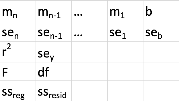
The explanation for each statistical variable mentioned in the array is as follows.
| Statistical Variable | Explanation |
|---|---|
| mn, mn-1, …, m1 | The slope for each independent variable (x) in the linear regression equation |
| b | The intercept of the linear regression equation you have |
| sen, sen-1, …, se1 | Standard error value for each slope coefficient (m) |
| seb | Standard error value for each intercept constant (b) |
| r2 | Determination coefficient. It determines whether the ability of x variables to predict the y variable can be trusted. The value is 0 to 1 and the closer the value is to 1, the more trusted the y prediction is |
| sey | Standard error value of the y prediction |
| F | The F-statistic value. It determines whether the relationship between x and y in the linear regression equation is random or not |
| df | Degrees of freedom. It is a support value to lookup the F-critical value of our linear regression equation in the statistical table. We will compare the F-critical value with the F-statistic value to determine the equation’s level of confidence. The larger the F-statistic value is compared to the F-critical value, the higher the level of confidence is |
| ssreg | Regression sum of squares. It determines the fitness of our equation with the data. The larger the regression sum of squares is, the more unfit the equation is with the data |
| ssresid | Residual sum of squares. It determines how much y cannot be predicted by our linear regression equation. The larger the residual sum of squares, the more unpredictable y we have |
Excel Version from Which LINEST can be Used
We can use LINEST since excel 2003.The Way to Write It and Its Result
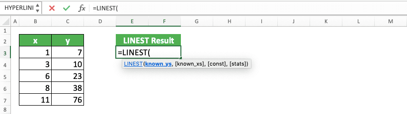
Generally, we can illustrate the way to write LINEST as follows.
=LINEST(known_ys, [known_xs], [const], [stats])
And here is a bit explanation for each input given in that writing.
- known_ys: the known dependent variables (y) values from the linear regression equation result
- [known_xs]: optional. The known independent variables (x) values from the linear regression equation. The number of x values must be balanced with the number of y values. If we don’t give input here, then it will assume x values are numbers from a progressive sequence starting from 1 (1, 2, 3, …)
- [const]: optional. The setting on the intercept value (b) calculation, whether LINEST should calculate it or not. If the input is TRUE, then it will be calculated and if FALSE, then the b value will be 0. If we don’t give input here, then it will be assumed as TRUE
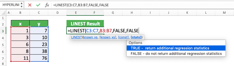
- [stats]: optional. The setting on the calculation of the statistical values besides the slope constant (m) and intercept (b). If the input is TRUE, then LINEST will calculate them and if FALSE, then it won’t. If we don’t give input here, then it will be assumed as FALSE
Example of Its Usage and Result
To make it clearer about the LINEST use, the following will give its implementation example and result in excel.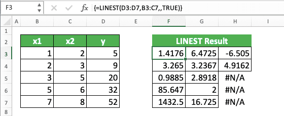
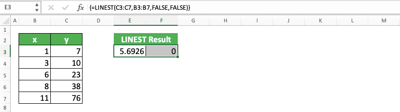
In the example, we can see how we write LINEST and the result we get from the writing. The LINEST writing usually uses an array formula form, symbolized by the curly brackets in front of and behind the writing. We can give an array form to a formula by pressing Ctrl + Shift + Enter buttons after we write it (we cannot type the curly brackets on our own).
If you want to get all values from the array result, don’t forget to highlight their cells before you write LINEST. If you don’t do it, then you will just get the first value from the array.
In the LINEST calculation on the example, we have two independent variables (x). In its input, we also specify that we want the statistical variables calculation results besides m and b too. As a result, we get all the values that you can see in the screenshot.
If we input FALSE in the LINEST’s last input, then we will only get three values in the example’s result. Those three values are slope constants (m) for x1 and x2 and also the intercept value (b).
Writing Steps
After discussing the LINEST implementation example, next, we will talk about the formula writing steps in detail. We will accompany the explanation for each step with its writing screenshot to make you understand the step easier.-
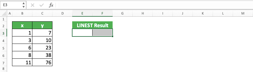
Highlight a cell range with the form and number of cells adjusted to the LINEST result you expect (look at the previous LINEST result explanation as a rough guide). Highlight the cell range in the place where you want to put the LINEST result
-
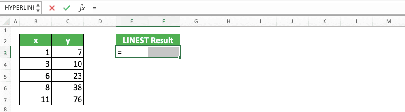
Type an equal sign ( = )
-
Type LINEST (can be with small and/or capital letters) and an open bracket sign
-
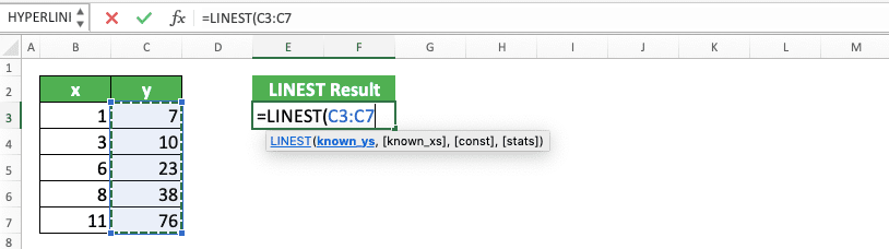
Input the cell range where the y variable values are. If you want to type the values directly, don’t forget to add curly bracket signs ( { } ) in front of and behind the typing
-
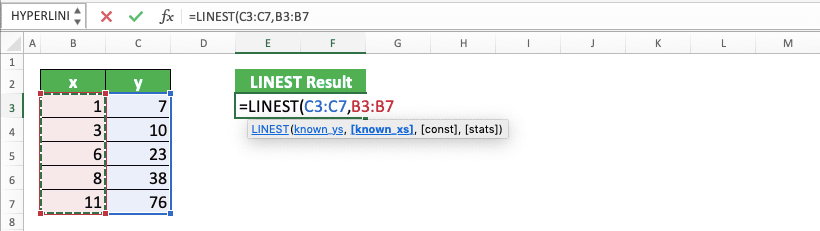
Optional: Type a comma sign ( , ) and input the cell range where your x variable(s) are. If you want to type them directly, don’t forget to type curly bracket signs in front of and behind the typing. If you don’t give input in this part, then the x values will be assumed as progressive numbers from 1 (1, 2, 3, …)
-
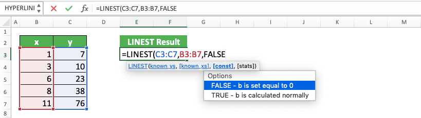
Optional: Type a comma sign ( , ) and type TRUE/FALSE to determine whether LINEST will calculate the intercept value (b). Type TRUE if you want to calculate it and type FALSE if you want to make 0 as the b value. If you don’t give input here, then it will assume your input as TRUE
-
Optional: Type a comma sign ( , ) and type TRUE/FALSE to determine whether LINEST needs to produce statistical values besides m and b. Type TRUE if yes and type FALSE if no. If you don’t give input here, then it will assume your input as FALSE
-
Type a close bracket sign
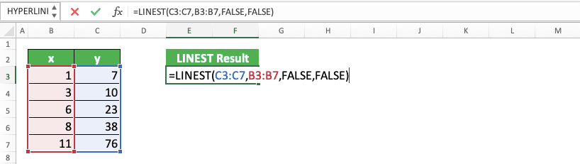
- Press Ctrl + Shift + Enter simultaneously to give an array formula form in your LINEST writing
-
Done!
General Reasons Why Your LINEST Gives a Wrong/Error Result
The LINEST you write gives a wrong or error result? Various possibilities can cause that. However, some factors that often become the main problems are as follows.- The unbalance of the x and y variables values inputs in your LINEST. This can cause a #REF, an error produced because of the formula references. Make sure the number of x values you give as its input balances the number of y values (your x values should be 5, 10, 15, etc. if there are 5 y values. It depends on how many x variables you have in your linear regression equation)
- You haven’t highlighted the cell range where you want to put the LINEST result correctly. This causes some of your LINEST calculation results to not show up. So, don’t forget to adjust the cell range highlight for your result according to the result you expect from LINEST
- Forget to press Ctrl + Shift + Enter buttons after you type your LINEST. This causes LINEST to not give all of its results
Make sure you don’t do those mistakes when you use LINEST!
How to Get a y Prediction from Your Linear Regression Equation Directly: SUM LINEST
What if we want to get a y value prediction from our LINEST result? Obviously, we can write the linear regression equation ourselves after getting the m and b values from LINEST. However, to make it easier, you can also use the combination of SUM and LINEST to predict your y.Generally, here is the writing form of SUM LINEST for this purpose.
=SUM(LINEST(y_values, [x_values], [need_b_or_not], [complete_result_or_not]) * {x1_value_to_predict_y, x2_value_to_predict_y, …, 1})
To predict y from a linear regression equation, we need its x values. These x values are combined with 1 in an array to then be multiplied with our LINEST result.
Because an array multiplication multiplies numbers in the same position, those x values are multiplied by m and 1 with b. From the multiplication, we will get the same calculation as the linear regression equation calculation, which is m1x1 + m2x2 + … + b. The summing process for the multiplication results is done by SUM which envelopes the multiplication process. The result is a y prediction based on the x values we want.
The number of x values input to predict y is adapted to the number of x variables in our equation. In this SUM LINEST formula writing, we don’t need an array formula form because the result we want is individual data.
To understand more about the SUM and LINEST combination for this y prediction, here is its implementation example in excel.
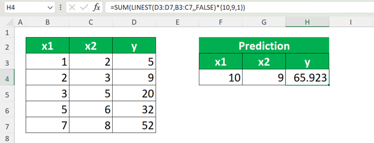
You can see in the screenshot’s formula bar, how we implement the SUM LINEST writing. As explained before, you need to write LINEST and the array, with x values and 1, in the SUM. With this writing, the calculation can run well and you can get the correct result.
Don’t forget to input x values according to the number of x variables. Don’t forget the number 1 in the array input also. If you input these wrongly, then you can get a #N/A error from your SUM LINEST writing.
An Alternative Way to Get the Intercept Value Individually: INTERCEPT/INDEX LINEST
Sometimes, when doing a calculation related to the linear regression equation. we might only need the intercept value (b). If that’s the situation, then we can use the INTERCEPT formula/INDEX LINEST combination to get the value individually (not in an array and with other values like the one you get when using LINEST)Generally, here is the way to write INTERCEPT to get that individual intercept value for you.
=INTERCEPT(y_values, x_values)
For INDEX LINEST, here is the general writing form.
=INDEX(LINEST(y_values, x_values), 2)
Unlike the normal LINEST writing, INTERCEPT and INDEX LINEST don’t need an array formula form. This is because both results are individual values and not several values in an array. Thus, you only need to press Enter, not Ctrl + Shift + Enter, after you finish writing one of them.
The x and y values inputted here is the same as the ones you input in LINEST. We input 2 in INDEX because the intercept value is in the second position in the LINEST array result.
As a note, you can only use INTERCEPT for a single linear regression equation (mx + b = y). If you need to get an intercept value from a multiple linear regression equation, then you should use INDEX LINEST.
To give an implementation and result example of both methods in excel, here is an example screenshot.
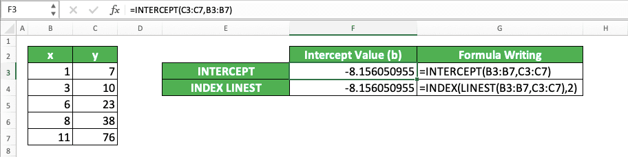
As you can see, both formula writings give the same result. As long as you correctly write the formula and correctly give the inputs, you will get the intercept value you need.
An Alternative Way to Get the Slope Value Individually: SLOPE/INDEX LINEST
What if the value you want to get individually is the slope constant (m)? You can use the SLOPE formula or INDEX LINEST which has been adjusted for its inputs. However, for this individual m calculation, we can only use INDEX LINEST for a single linear regression equation (not like in the intercept calculation before) like SLOPE.The SLOPE general writing form to get our slope constant value individually is as follows.
=SLOPE(y_values, x_values)
=INDEX(LINEST(y_values, x_values), 1)
Like the previous intercept value calculation, you don’t need an array formula form in both writings. We just need to press Enter, not Ctrl + Shift + Enter, when finishing the formula writing.
The inputs you need to give for both are the x and y values from your single linear regression equation. In the INDEX second input, we input 1 there because m is in the first position of a LINEST array result.
To make you understand it better, let’s see both implementation and result example in excel below.
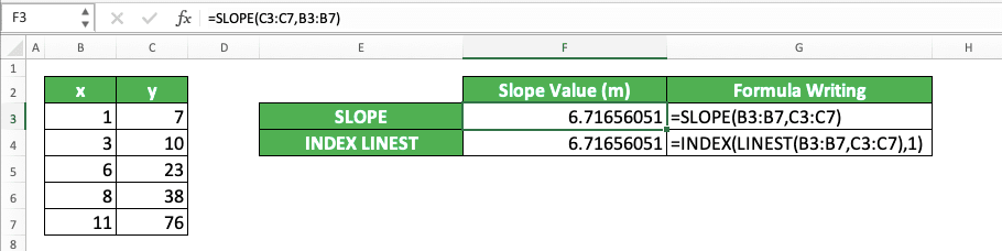
Same results, right? Just choose whichever formula writing you want to use when looking for the slope value of your single linear regression equation.
Exercise
After learning how to use LINEST in excel completely, let’s do an exercise. This is so you can understand more about the LINEST implementation in excel.Download the exercise file of the link below and answer all the questions. Download the answer key file if you have done the exercise or when you are confused to answer the questions!
Link of the exercise file:
Download here
Instructions
Use LINEST to find the answer to each question! Fill the answer in the appropriate gray-colored cell according to the question number!- What is the b value in the linear regression equation with those x and y values?
- What is the F value in the linear regression equation with those x and y values?
- What is the y value if x1, x2, and x3 are 10 each, based on the linear regression equation?
Link to the answer key file:
Download here
Additional Note
If you want to edit your LINEST writing, then you need to delete all content of the result cell range first. Because the LINEST result is an array, all its values are connected and cannot be edited one-by-one.Related tutorials you should learn too: