SUM Formula in Excel: Functions, Examples and How to Use
Home >> Excel Tutorials from Compute Expert >> Excel Formulas List >> SUM Formula in Excel: Functions, Examples and How to Use


In this tutorial, you will learn how to use the SUM formula/function in excel completely. We will discuss the basics of SUM and its advanced use too to optimize your numbers processing in excel.
The sum is a basic calculation process that many of us use to get the results we desire from our numbers. When we process our numbers in excel, SUM can help us to sum them fast. We can also combine SUM with many formulas to optimize its capabilities and run more complex data analysis.
Curious to learn more about SUM and what we should do with this formula? Read all parts of this complete SUM tutorial from Compute Expert!
Disclaimer: This post may contain affiliate links from which we earn commission from qualifying purchases/actions at no additional cost for you. Learn more
Want to work faster and easier in Excel? Install and use Excel add-ins! Read this article to know the best Excel add-ins to use according to us!
Table of Contents:
- What is SUM in Excel?
- SUM function in excel
- SUM result
- Excel version from which we can start using SUM formula in excel
- The way to write it and its inputs
- Example of its usage and result
- Writing steps
- Common factors why your SUM produces an error/wrong result
- Rounding process after SUM: ROUND/ROUNDUP/ROUNDDOWN SUM
- SUM the largest/smallest values: SUM LARGE/SMALL
- SUM based on a reference value: SUM VLOOKUP
- SUM a cell range which coordinate is based on cell values: SUM INDIRECT
- SUM to count data based on multiple criteria and OR logic: SUM COUNTIF
- SUM every nth row: SUM MOD ROW
- SUM a filtered cell range: SUBTOTAL
- SUM with IF: SUMIFS
- SUM with error values in its cell range input: SUM IFERROR
- Much faster SUM writing to sum a number sequence: AutoSum
- Exercise
- Additional note
What is SUM In Excel?
We can define SUM as an excel calculation function that can help us to sum numbers fast and accurately.SUM Function in Excel
We can use SUM to sum numbers from direct typing, cells, or cell ranges fast.SUM Result
SUM will give us a number which is the total of all the numbers we input into it.Excel Version from Which We Can Start Using SUM Formula in Excel
We can start using SUM in excel 2003.The Way to Write It and Its Inputs
Here is the general writing form of the SUM function in excel.
= SUM ( number1 , number2 , … )
The numbers we input into SUM can be in the forms of direct typing, cell coordinates, or cell ranges. However, we usually only input one cell range to SUM which contains all the numbers we want to process.
Remember to type comma signs ( , ) between the inputs we give to SUM.
Example of Its Usage and Result
Here is the implementation example of SUM in excel. You can see the writing and the result of the formula here.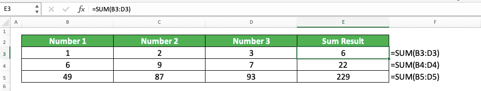
In the example, we want to sum the numbers in each row. We use the SUM formula to help us run the sum process easier.
The way to use SUM is quite easy. Just input the numbers we want to sum into the formula. Here, as the numbers are all in each row cell range, we just input those row cell ranges into our SUM.
Write the SUM formula correctly, enter, and we will immediately get the sum result of our numbers!
Writing Steps
After we discuss the writing form, inputs, and example of SUM, now we discuss its writing steps in excel. If you have understood the tutorial discussion earlier, then you should be able to follow these steps with no problem!-
Type an equal sign ( = ) in the cell where you want to put the sum result of your numbers
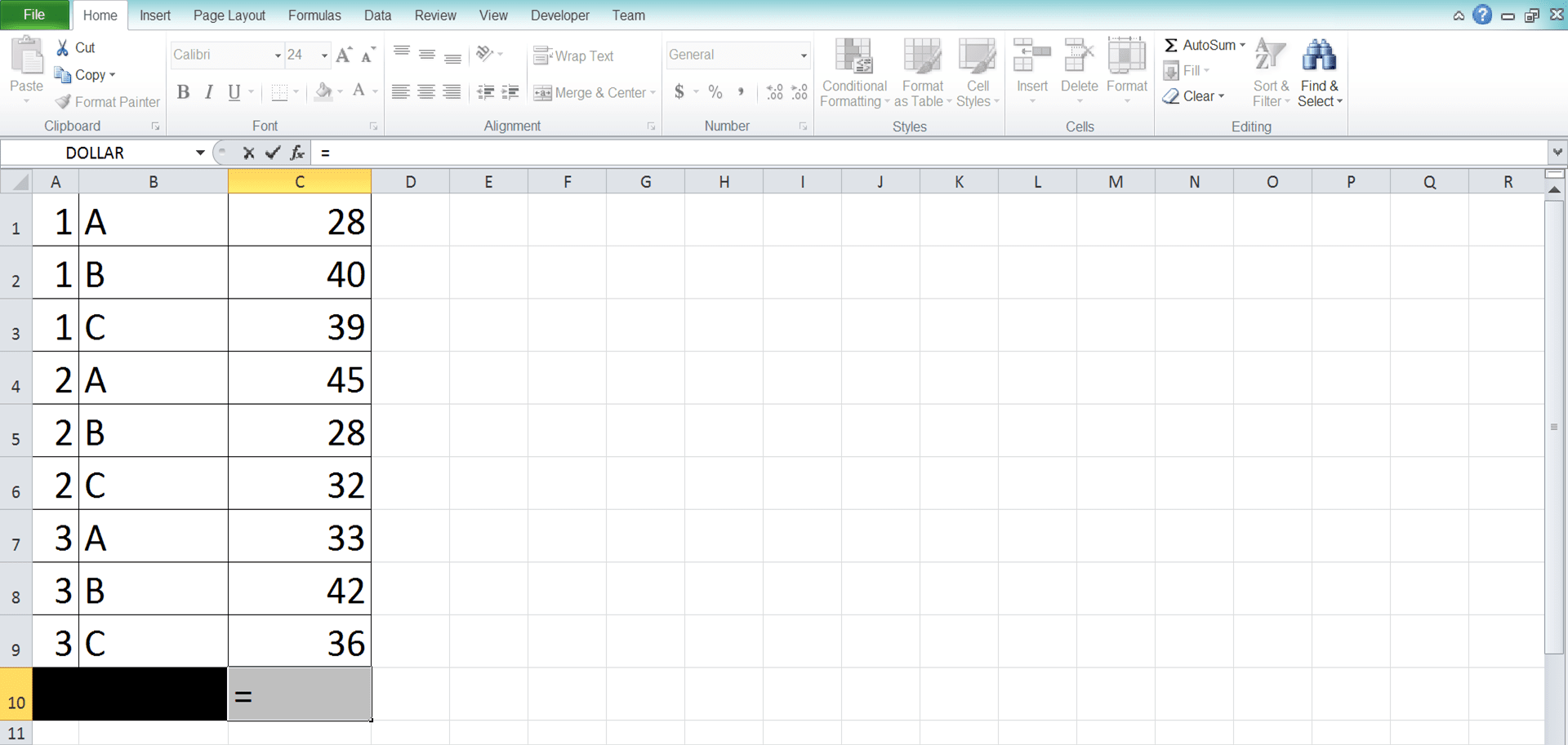
-
Type SUM (can be with large and small letters) and an open bracket sign after =
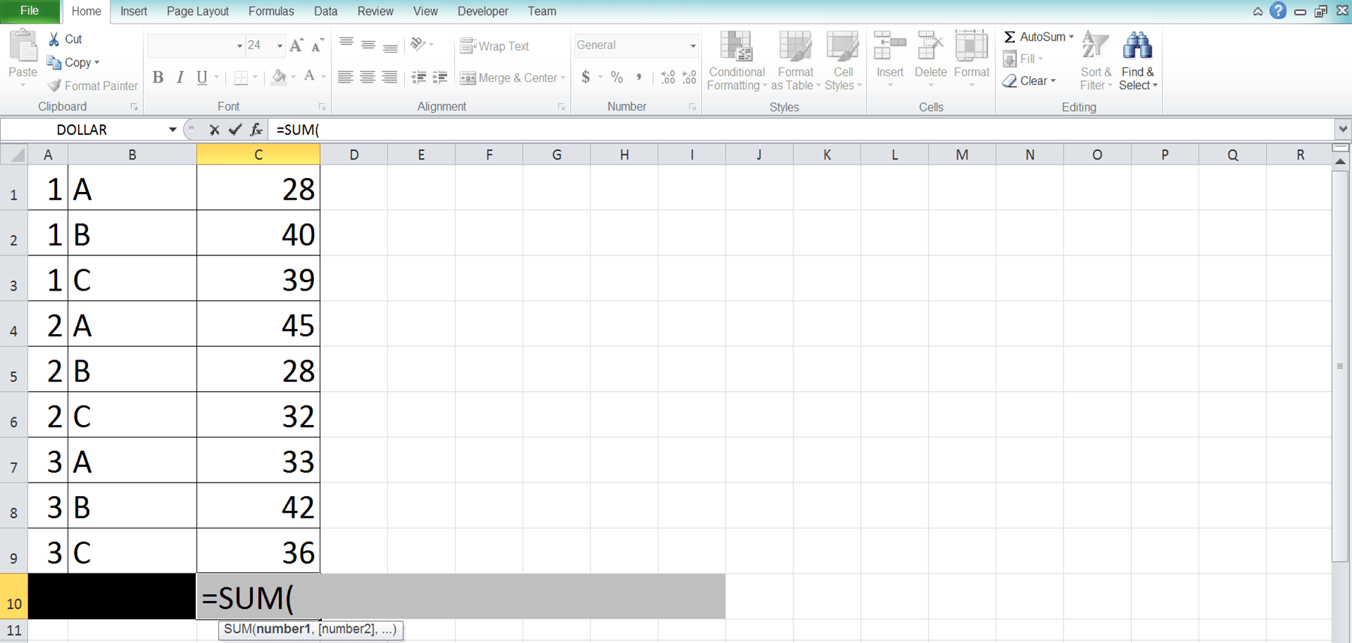
-
Input all the numbers you want to sum in the forms of direct typing, cell coordinates, and/or cell ranges. If you give more than one input, then separate them with comma signs

-
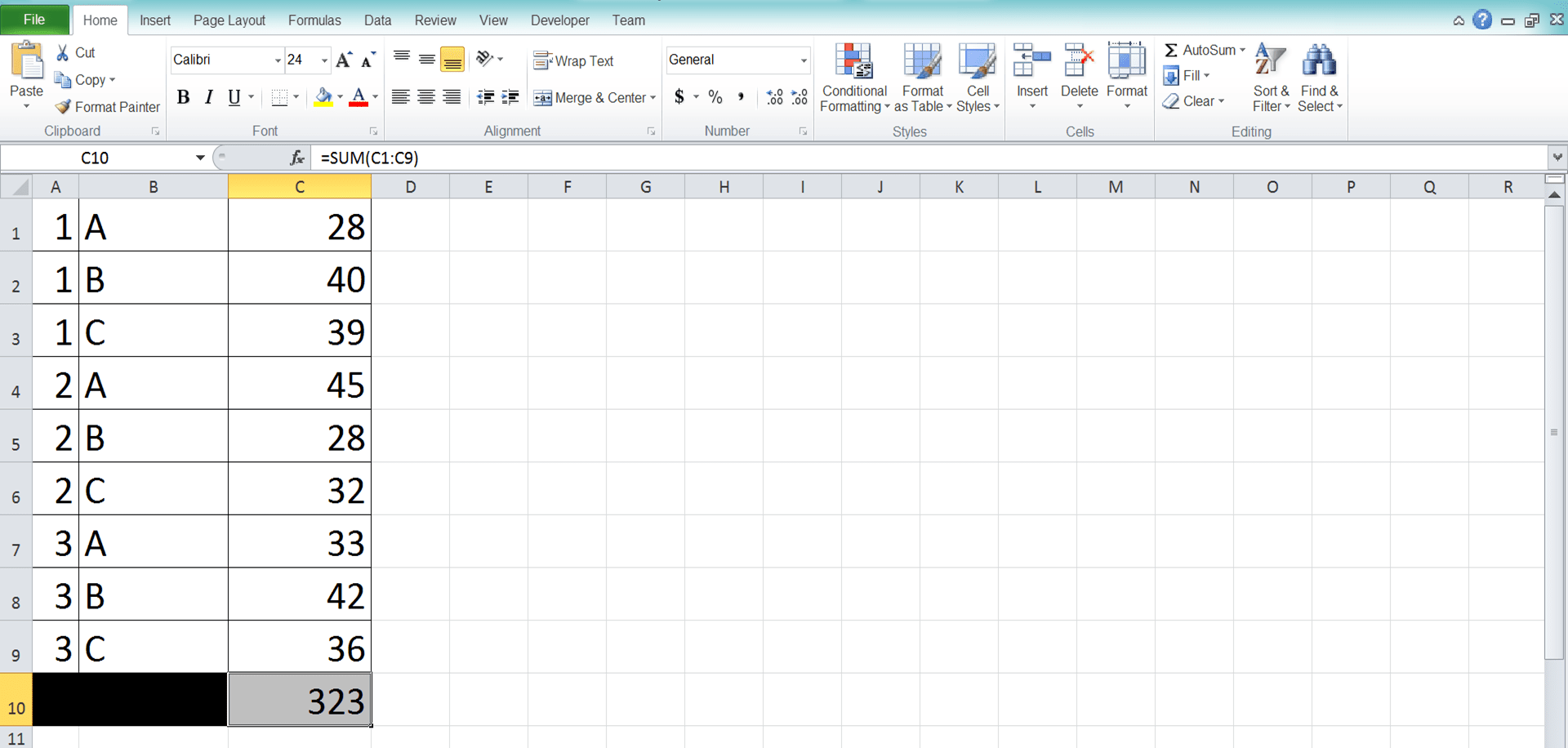
Type a close bracket sign after you have inputted all the numbers you want to sum

- Press Enter
-
Done!
Common Factors Why Your SUM Produces an Error/Wrong Result
Your SUM gives you an error/wrong sum result? Check your SUM writing with the guidance of these points below!- You give more or fewer inputs than you need to get the correct SUM result. This sometimes happens when you need to sum many numbers. Check again your input to make sure you have given the correct numbers
- Your SUM inputs probably contain some different kinds of numbers like dates, percentages, time, etc. These inputs can make SUM produces an unexpected result for you
- Your SUM inputs might contain some error values (if this is the case, then most probably they are in the cell ranges that you input). These values can make your SUM produces an error too. If you want SUM to ignore those errors, see how to do this in the SUM IFERROR part of this tutorial
Rounding Process after SUM: ROUND/ROUNDUP/ROUNDDOWN SUM
After you get your SUM result, especially if you sum decimals, you may need to round it. To do that immediately, you can combine SUM writing with excel decimal rounding formulas: ROUND/ROUNDUP/ROUNDDOWN.You can combine those formulas with SUM quite easily too. Just write SUM inside the rounding formula you use. Write it as the number-to-round input in the rounding formula.
To summarize, here is the general writing form of the formulas’ combination in excel.
= ROUND / ROUNDUP / ROUNDDOWN ( SUM ( number1 , number2 , … ) , number_of_decimals )
Regarding the formula you should use, here is what each decimal rounding formula does to your SUM result.
- ROUND = round your SUM result normally (will round 0-4 numbers down and 5-9 numbers up)
- ROUNDUP = round up your SUM result
- ROUNDDOWN = round down your SUM result
Choose the rounding formula according to the need of your final result!
To understand the concept of this rounding formula + SUM combination easier, here is the implementation example in excel.

In the example, we have some decimals we want to sum on each row. As we want to round the sum result immediately, we can combine SUM with ROUND/ROUNDUP/ROUNDDOWN in one formula writing.
Just input the SUM in the decimal rounding formula we choose. Don’t forget to input the number of decimals we want for the result too.
Additionally, you can also round to powered ten multiples (10, 100, 1000, etc) using ROUND/ROUNDUP/ROUNDDOWN. Just input a negative number in your rounding formula’s number of decimals input. Determine the negative number value according to the power level you want to give for the 10 multiples (1 for 10, 2 for 100, 3 for 1000, etc).
SUM the Largest/Smallest Values: SUM LARGE/SMALL
Need to sum the largest/smallest values in the group of numbers that you have? To do it in one formula writing, you can combine SUM with LARGE (for the largest values)/SMALL (for the smallest values).If you have used LARGE/SMALL before, then you know we usually only get one nth largest/smallest value from it. However, if you input an array in the formula nth largest/smallest input, then you can get an array result too. We can use this fact to make SUM directly sum the largest/smallest values in our group of numbers.
Here is the general writing form of the SUM and LARGE/SMALL combination.
= SUM ( LARGE/SMALL ( numbers_cell_range , { nth1 , nth2 , … } ) )
You can determine how many top/bottom values you want to sum in the LARGE/SMALL’s nth largest/smallest array input. For example, if you want to sum five top values from your numbers, then you can input {1,2,3,4,5} to your LARGE.
You can also input the array to LARGE/SMALL in the form of a cell range. For this, however, you need to use the array formula form so your LARGE/SMALL can process it correctly. To use the array formula form, press Ctrl + Shift + Enter after you finish writing your formula instead of Enter only.
Here is the implementation example of the SUM and LARGE/SMALL formulas combination in excel.
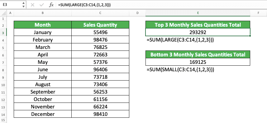
In the example, we have monthly sales quantities data. We want to know the total of the top 3 and the bottom 3 separately. To easily do the calculation, we use SUM and LARGE/SMALL.
We input our LARGE/SMALL in our SUM and input the monthly sales quantity cell range in the LARGE/SMALL. For the second input of the LARGE/SMALL, we input a {1,2,3} array. That is because we want to sum the first, second, and third-largest/smallest numbers.
We do the writing like that and we can sum the top 3 and bottom 3 monthly sales quantities fast!
SUM Based on a Reference Value: SUM VLOOKUP
Let’s say you have a reference table containing numbers and you want to sum numbers that belong to a certain variable. Can we pull those numbers from the table and sum them using SUM?The answer is yes, you can. However, to do that in one writing, you need to combine your SUM with VLOOKUP.
Here is the general writing of the SUM and VLOOKUP combination for that sum process.
{ = SUM ( VLOOKUP ( variable_to_sum , reference_table_range , { column_to_sum1 , column_to_sum2 , … } , lookup_mode ) }
In this SUM and VLOOKUP combination, we use VLOOKUP to pull the numbers we want to sum from a certain variable. We input the variable as our lookup reference and the reference table cell range too in VLOOKUP.
For the VLOOKUP result column index input, we input an array that contains all the column indexes we want to sum. The index starts from 2 since the first one belongs to the variable column range. We need to input all column indexes in the reference table if we want to sum them all.
We can use TRUE or FALSE for the VLOOKUP lookup mode input depending on the lookup process we want to do. As usual, input TRUE to enable an approximate match search and FALSE for an exact match search.
Input all of those VLOOKUP writings to SUM. In the formula writing, we use an array formula form (the curly bracket signs that envelop the formula are the sign for the array formula form) since our VLOOKUP needs to deal with an array input. Because of this, we need to press Ctrl + Shift + Enter after we write the formula instead of just Enter (to change our formula form into an array formula).
Here is the implementation example of the SUM and VLOOKUP combination.
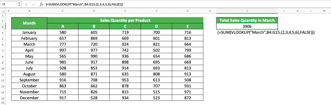
In the example, we have a table of monthly sales quantity data for five products. If we want to get one month’s sales quantities total from the table, then we can use SUM and VLOOKUP combination.
Just write the SUM and VLOOKUP in the way we discussed earlier. Input the month (March for this example), the reference table cell range, and column indexes array into our VLOOKUP. We input FALSE as the lookup mode here since we want to sum only the March sales quantities.
Write the VLOOKUP with these inputs into SUM and press Ctrl + Shift + Enter. We will immediately get the total sales quantity for March!
SUM a Cell Range Which Coordinates Are Based on Cell Values: SUM INDIRECT
Want to determine the row/column you use your SUM on based on cell values? If you want your SUM cell range input to be dynamic like this, then you can combine it with INDIRECT.INDIRECT is an excel formula that can convert a regular text into a cell reference. For example, if you write =INDIRECT(“C5”) in a cell, then that cell value will refer to the cell C5 value. This is an excellent formula to use whenever you need to make a formula’s cell/cell range references to constantly changes.
The usual way to write a SUM and INDIRECT combination for a dynamic SUM input itself is like this.
= SUM ( INDIRECT ( column_letter1 & row_number1 & “:” & column_letter2 & row_number2 ) )
Input cell coordinates to the column letter and row number inputs you want to refer to cell values in the INDIRECT.
Input from where you want to sum in the first pair of your column letter and row number. Next, input to where you want to sum in the second one. This mirrors the cell range reference form in excel where we write the first cell, colon, and the last cell (for example, A1:C5 means we refer to cell A1 to cell C5).
By correctly inputting to INDIRECT, you can change the cell range you refer in your SUM by changing your cell values!
You can see the implementation example of the SUM and INDIRECT combination below.
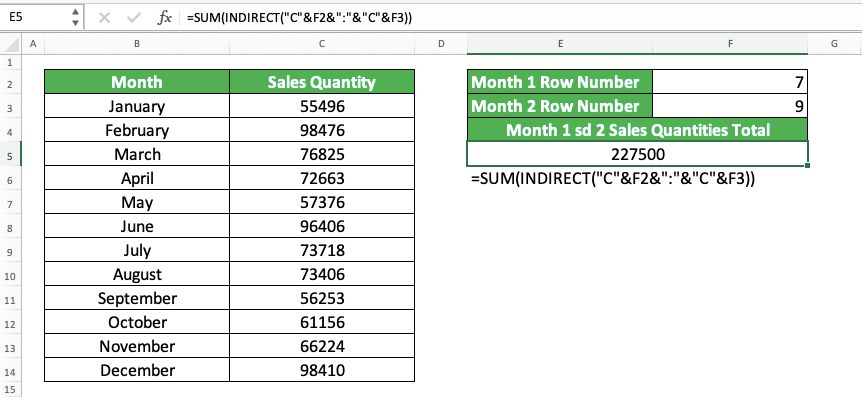
Here, we want to determine the month range we want to sum the sales quantities on based on cell values. We can use the combination of SUM and INDIRECT for that.
Just write an INDIRECT inside your SUM with the inputs of appropriate column letters and row numbers. Since the monthly sales quantity numbers are all in column C, we can just input “C” for our column letter inputs.
For the to and from row numbers, we refer to cell values as you can see in the screenshot. Because of this, we can change the cell range reference in SUM by just changing the cell values we refer to.
SUM to Count Data Based on Multiple Criteria and OR Logic: SUM COUNTIF
We can combine SUM with many other formulas in excel for various purposes. We have seen some examples of them earlier. Another one here is combining SUM with COUNTIF to count data using multiple criteria with OR logic.COUNTIF is a formula we can use to count data based on a criterion we have. However, it cannot count data using multiple criteria and OR logic by itself (its sibling formula, COUNTIFS, count data using multiple criteria but with an AND logic). OR logic here means we want to count all data that fulfill at least one of our criteria.
However, by combining it with SUM, we can do that OR counting process. Here is the general writing form of SUM and COUNTIF for this purpose.
= SUM ( COUNTIF ( cell_range1 , criterion1 ) , COUNTIF ( cell_range2 , criterion2 ) , … ) )
In this writing, SUM will sum the data amount in your cell ranges that matches one of your criteria. Input the number of COUNTIFs into your SUM that matches the number of criteria you have. The cell ranges you input to your COUNTIFs can be the same or different depending on your needs.
Here is the implementation example of the SUM and COUNTIF combination for the data counting purpose.
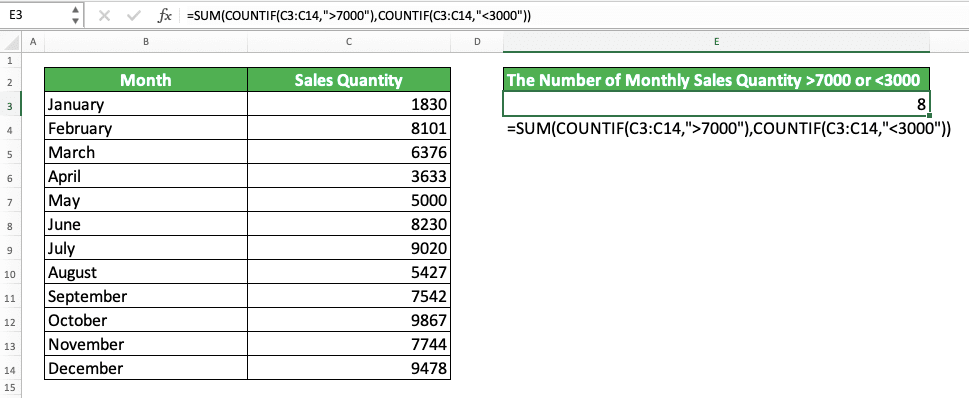
In this example, we count the number of monthly sales quantities that are more than 7000 or less than 3000. We use a SUM and COUNTIFs combination to make the data counting process faster.
Since we have two criteria here, we use two COUNTIFs in our SUM. The data we want to count is in the same cell range for both criteria. Therefore, we input the same cell range for the COUNTIFs in this example (the sales quantity column cell range).
We get the COUNTIF result for each criterion and we sum them using SUM. By doing this, we can get our data counting result with multiple criteria and OR logic!
SUM Every Nth Row: SUM MOD ROW
Sometimes, we probably don’t want to sum all of the numbers we have in a column. We may only need to sum the numbers in every nth row instead.Using SUM alone isn’t enough when we have this situation. To help us adding the numbers in every nth row, we should use the combination of SUM, MOD, and ROW.
You may have known and utilized the functions of MOD and ROW before in excel. We can use MOD to get a division process remainder while ROW gives us the row number of a cell. Combining them with SUM can give us the ability to loop through numbers in rows in our sum process.
The general writing form of the SUM, MOD, and ROW combination is as follows.
{ = SUM ( numbers_range * MOD ( ROW ( appropriate_similar_sized_range_to_numbers_range ) , nth_row ) = 0 ) }
We will explain the process that runs in the formula writing by using the help of the example below.
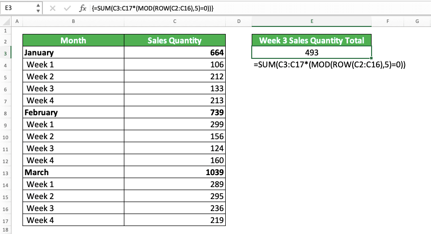
In the example, we have a monthly and weekly sales quantity table. We want to sum only the week 3 sales quantities from the table. Therefore, we should use a SUM, MOD, and ROW combination.
To get only the sales quantities from week 3, we multiply the sales quantity column with MOD and ROW in SUM. We use MOD and ROW here to get a TRUE and FALSE array that will filter the week 3 sales quantities.
We input an appropriate same-sized cell range to our ROW to get the TRUE and FALSE array. We base the cell range input on the nth row we want to get from the sales quantity column.
We aim to get 0 from the MOD and ROW result for the week 3 rows in the sales quantity column. That is because we have an “equal to 0” condition at the end of our MOD.
The 0 will produce a TRUE logic value while other numbers will produce FALSE logic values because of that condition. As TRUE is 1 and FALSE is 0 in excel, our multiplication with the sales quantity column will produce as follows. All the sales quantities we multiply will become 0 from rows other than week 3 rows!
As week 3 has five rows distance and it starts in the fourth row, we input ROW the C2:C16 range. The C2:C16 has an equal size to the sales quantity column (C3:C17). It also makes week 3 rows produce 5 from ROW and thus, become 0 when we divide them with MOD.
To summarize the results chronology, from the ROW formula we write in the example, we get this array result.
{ 2 , 3 , 4 , 5 , 6 , 7 , 8 , 9 , 10 , 11 , 12 , 13 , 14 , 15 , 16 }
The 5 multiples there are in parallel with the week 3 numbers. This is important to make them not become 0 in our multiplication process later.
We divide all those array numbers with 5 we input to our MOD and we get this.
{ 2 , 3 , 4 , 0 , 1 , 2 , 3 , 4 , 0 , 1 , 2 , 3 , 4 , 0 , 1 }
As we compare the MOD result with 0 in our formula writing, we get this from the comparison result.
{ FALSE , FALSE , FALSE , TRUE , FALSE , FALSE , FALSE , FALSE , TRUE , FALSE , FALSE , FALSE , FALSE , TRUE , FALSE }
Which, in excel calculation, is similar to this.
{ 0 , 0 , 0 , 1 , 0 , 0 , 0 , 0 , 1 , 0 , 0 , 0 , 0 , 1 , 0 }
We multiply this array to the sales quantity numbers in our column. From that multiplication, we get this number array.
{ 0 , 0 , 0 , 133 , 0 , 0 , 0 , 0 , 124 , 0 , 0 , 0 , 0 , 236 , 0 }
Notice that only the week 3 sales quantity numbers are not 0.
We sum the numbers in the array using SUM. From this, we get the week 3 sales quantities total, which is 493!
Don’t forget the array formula form for this SUM, MOD, and ROW combination too. As we input an array to our ROW, we must press Ctrl + Shift + Enter after we write our formula.
SUM a Filtered Cell Range: SUBTOTAL
If we apply SUM to a filtered cell range, then it will sum the numbers that don’t pass our filter too. To sum only the numbers that pass, we should use SUBTOTAL instead.SUBTOTAL is an excel formula that specializes itself in processing data that passes filters. We can use several formulas through SUBTOTAL for our filtered data, including SUM.
Here is the SUBTOTAL general writing form if we want to sum numbers in a filtered cell range.
= SUBTOTAL ( 9 / 109 , filtered_range1 , filtered_range2 , … )
The 9 or 109 input there is the SUM formula code number when we use SUBTOTAL. We use 9 if we want to sum the numbers in the cells we hide manually too in the filtered ranges. If we want to ignore them, then we input 109.
In SUBTOTAL, we can input multiple filtered cell ranges for our SUM calculation after the 9/109 input. However, most of the time, we only input one filtered range. If we happen to input multiple filtered ranges, then don’t forget to separate them with commas.
To better understand the SUBTOTAL implementation to apply SUM in a filtered cell range, look at the example below.
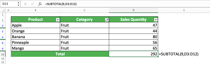
In the example, we have a filtered cell range and we want to sum the numbers that pass the filter there. This is a perfect situation example to use SUBTOTAL in excel.
We input 9/109 as the formula code input in SUBTOTAL to conjure SUM. In this example, it doesn’t matter we input 9 or 109 since we don’t have manually hidden cells in the range. We will produce the same sum result using either code.
We give the code input and the filtered cell range to our SUBTOTAL. As a result, we get a SUM result from the numbers that pass our filter! If you happen to change the filter in the cell range, then the SUBTOTAL result should change too!
SUM with IF: SUMIFS
We have discussed quite a bit about COUNTIF as the excel formula to count data that passes a criterion. But, what if we want to sum the numbers from the data entries that pass the criteria that we have?Can we do a SUM with an IF-like function like that? For this one, we can use a variant formula from SUM, which is SUMIFS.
Here is the general writing form of SUMIFS in excel.
= SUMIFS ( number_range , data_range1 , criterion1 , data_range2 , criterion2 , … )
In SUMIFS, we input the cell ranges where our data entry numbers are and data with the criteria that evaluate them. We input the data cell range and the criteria in pairs. This means a criterion will only evaluate the data in the cell range we input before it.
The cell ranges we input in SUMIFS should be parallel and have the same size. Usually, we input them in the form of columns/rows.
To better understand the SUMIFS implementation in excel, here is a screenshot example.
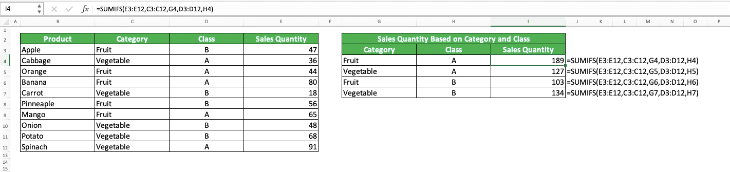
We have fruits and vegetable sales quantity data in a table in the example. On the right, we want to sum the sales quantities based on the product category and class. For this kind of sum process, we can use SUMIFS to help us get our results.
First, we input the sales quantity column cell range for our numbers range input in SUMIFS. As we have product category and class criteria for the sum process, we input the relevant data cell ranges and criteria.
In the example, we input the category column cell range first and its criterion. Then, we input the product class column cell range and its criterion.
Write the SUMIFS correctly and give it correct inputs according to our sum needs. In the example, as a result of this, we get all of the SUMIFS results we need correctly!
SUM with Error Values in its Cell Range Input: SUM IFERROR
Error values in a SUM cell range input are one factor that can cause our SUM to produce an error. We should remove error values from our cell range so we can get the correct sum result from SUM.But, what if we cannot predict the error values that might show up in our cell range (probably they come from excel formula results which has dynamic inputs)? What if we have a large cell range and it will be troublesome to inspect and remove all errors?
In these kinds of situations, we can combine our SUM with IFERROR. That way, we can use SUM to our cell range without any worry about its error values!
The general writing form of SUM and IFERROR combination for the purpose is like this.
{ = SUM ( IFERROR ( numbers_range , 0 ) ) }
In this combination, we write our IFERROR in our SUM and input our numbers range to the IFERROR.
As a substitute for each error that we have, we input 0 in our IFERROR. However, if you want, you can substitute the error values with any value you prefer. Just change the 0 in your formula writing with the value you want.
Because IFERROR receives an array input (in the form of the number range) and we expect it to produce an array result (it usually receives an individual input and produces an individual data), we use an array formula form. Therefore, we need to press Ctrl + Shift + Enter after we write the formula, not just Enter as usual.
You can see the implementation example of the SUM and IFERROR combination in the screenshot below.
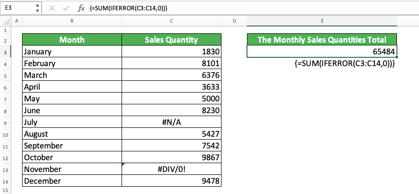
In this example, we want to sum all the monthly sales quantity numbers we have in our table. However, as you can see, there are two error values there (#N/A and #DIV/0). If we want to sum the numbers without removing the errors, then we can combine SUM with IFERROR to do it.
We input the sales quantity column cell range into our IFERROR and we input the IFERROR into our SUM. Here, we substitute all the error values in the sales quantity column with zeroes.
After we finish writing the formula, we press Ctrl + Shift + Enter to convert it into an array formula. As a result, we get the sales quantity numbers total while ignoring several errors in it!
Much Faster SUM Writing to Sum a Number Sequence: AutoSum
Do you know there is a SUM writing shortcut you can use to a number sequence in excel? The feature to access this shortcut is what we call AutoSum. If you often sum numbers in excel, then this feature can make you sum much faster.To understand how to use this feature, see the example below.
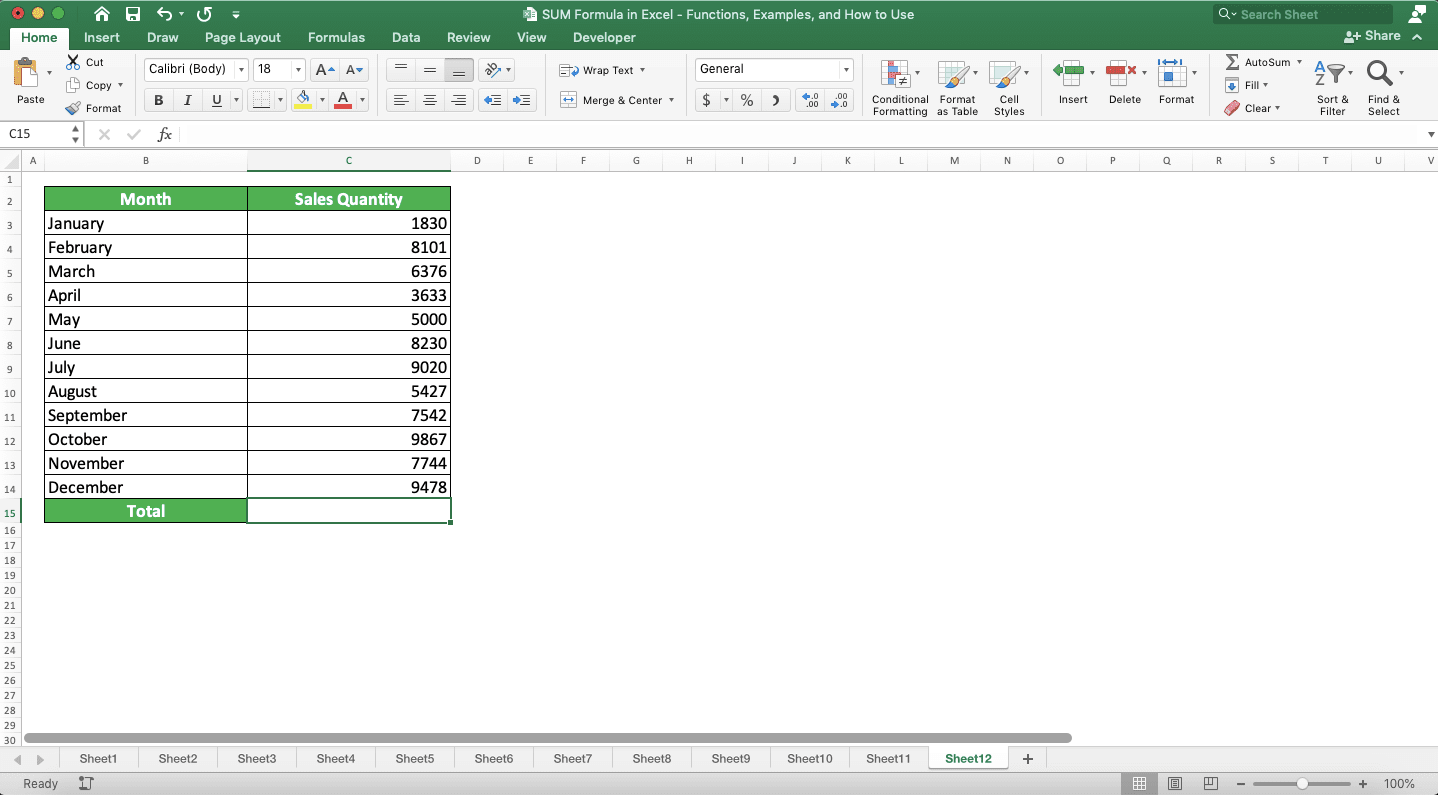
We use the monthly sales quantity data set we have used previously for this AutoSum implementation example. Now, how to use the feature to sum the sales quantity numbers fast?
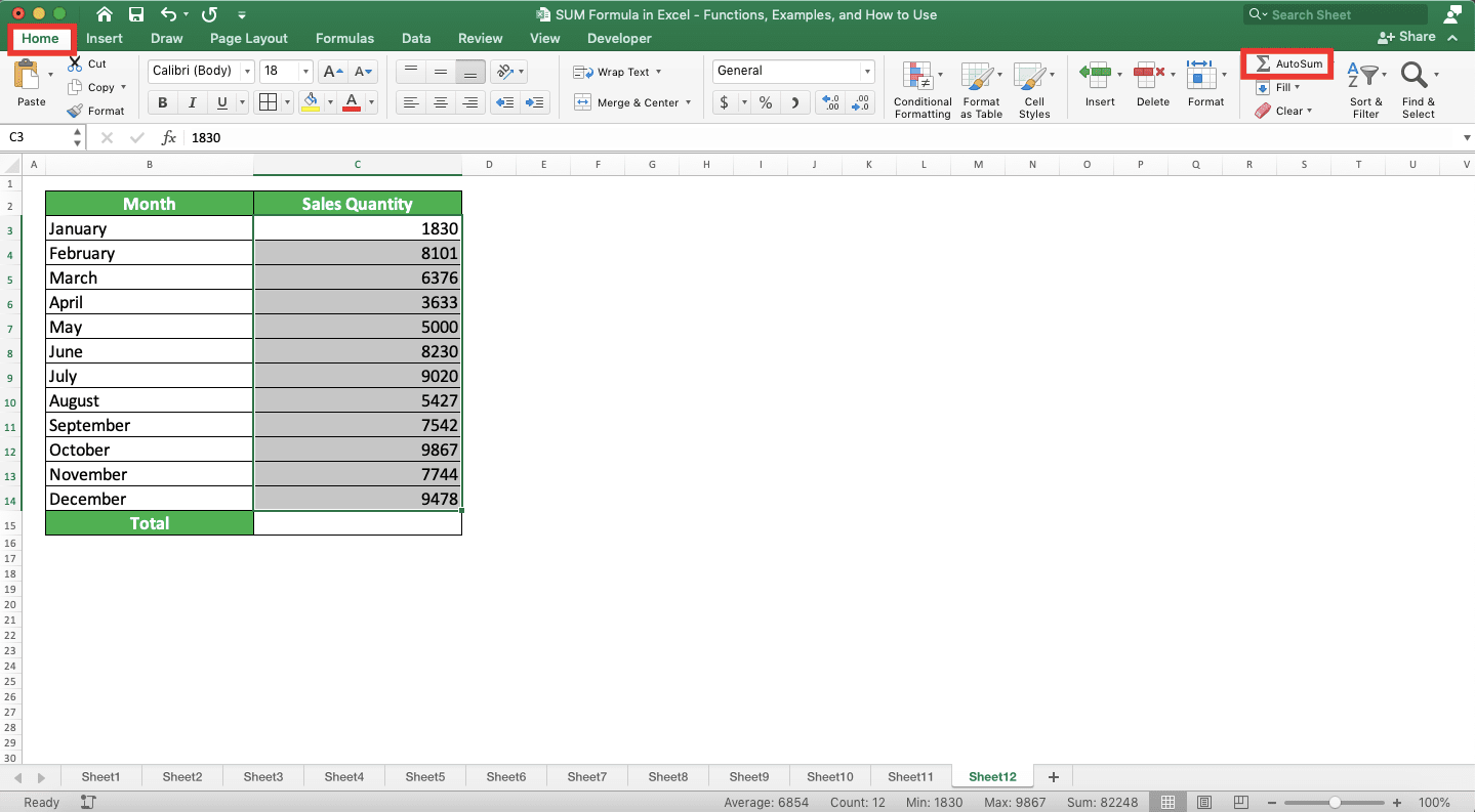
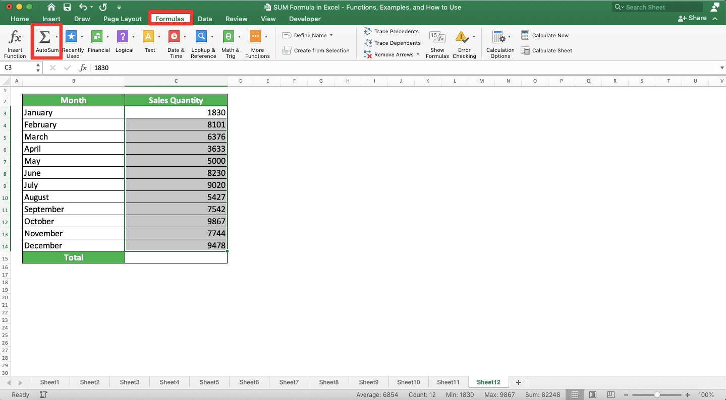
First, we highlight the sales quantity number sequence or we place our cell cursor just outside those numbers. Then, we go to the Home or the Formulas tab and click the AutoSum button. We can also press the AutoSum shortcut buttons, Alt + = (Command + Shift + T in Mac).
AutoSum button in the Home tab
AutoSum button in the Formulas tab
After you run the AutoSum feature, excel will automatically write a SUM to sum your number sequence!
Now, you don’t have to write SUM yourself when you want to sum a number sequence in excel!
Exercise
After you have learned how to use the SUM formula in excel completely, let’s do an exercise. This is so you can understand the lessons you get from this tutorial more practically.Download the exercise file from the following link and answer the questions below. Download the answer key file if you have done the exercise and want to check your answers.
Link to the exercise file:
Download here
Questions
- What is the SUM result of all numbers in the first column?
- What is the SUM result of all numbers in the second column? Avoid black colored cells when you give the number inputs to your SUM
- What is the SUM result of all numbers in the third column? Avoid black colored cells when you give the number inputs to your SUM
Link to the answer key file:
Download here
Additional Note
- SUM ignores text and blank cells in its sum process
- You can give up to 255 different inputs to SUM
Related tutorials you should learn: