How to Count Data in Excel: Formulas and Functions

In this tutorial, you will learn how to count data in excel.

Often, the data counting process that we need to do in excel has some specifications. There will be various methods and formulas or formulas combination given here that can help us do it. One of them, at the very least, should be able to answer your need to count data in excel.

Disclaimer: This article has affiliate links that might give us commission, without any additional cost to you. All of the affiliate links here offer products/services that can help you use excel more optimally in your daily work. If you want to read further about this, you can visit our Affiliate Disclosure page.

Disclaimer: This post may contain affiliate links from which we earn commission from qualifying purchases/actions at no additional cost for you. Learn more

Want to work faster and easier in Excel? Install and use Excel add-ins! Read this article to know the best Excel add-ins to use according to us!

A Brief Explanation of Various Data Counting Formulas in Excel and Their Functions

There are various formulas or formula combinations you can use to count data in excel. Their uses, of course, depend on your data processing needs and the kind of data you want to count.

Excel provides 5 formulas for its data counting process:

• COUNT, useful to count the number of numbers in a cell range
• COUNTA, useful to count the amount of data in a cell range
• COUNTBLANK, useful to count the number of blank cells in a cell range
• COUNTIF, useful to count the amount of data that fulfill a particular criterion in a cell range
• COUNTIFS, useful to count the amount of data/data entries that fulfill criteria

If you need other data counting besides the ones mentioned above, then you must use formula combinations or other methods.

In the next parts of this tutorial, we will discuss various ways to count data in excel specifically. Either using formulas provided by excel or using other methods.

Count the Number of Cells With Numbers: COUNT

The first count method we discuss is COUNT. COUNT is useful to count how many numbers you have in a cell range.

This formula is quite easy because you just need to input data/cells/cell ranges. The input is where you want to count your numbers. Generally, here is the writing illustration of COUNT:



Although you can input many things in COUNT, usually we just input a cell range in it. However, if needed, you can also input more than one cell range or data or cell coordinate.

The following is the example of COUNT’s usage and result in excel.



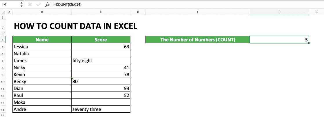
As you can see there, COUNT counts the number of pure numbers in its cell range/cell/data input. It doesn’t count numbers with text data type or number in words.

The writing you see in the formula bar is the example of COUNT writing that is often used. As mentioned before, we usually just input a cell range in it. COUNT will then count how many numbers are there in that cell range.

If you want to learn deeper about COUNT, please visit this tutorial.

Count the Number of Cells With Data: COUNTA

What if we don’t want to just count numbers, but also other types of data in a cell range/cell/data? For that need, we can use the COUNTA formula.

Generally, the COUNTA writing in excel can be illustrated as follows.



Like COUNT, usually, we just input one cell range in COUNTA. From the cell range, COUNTA will count how many cells are filled with data in it, to then produce its result.

For a clearer understanding of COUNTA, here is an example of its usage and result in excel.



In the example, we can see how COUNTA gives the amount of data in the score column’s cell range. Because there are 8 cells filled with data there, COUNTA gives 8 as its result to us.

As a note, COUNTA also counts errors and formulas that produce blank data (usually symbolized with two quotes (“”)) in its data counting process.

If you want to know more about COUNTA, please visit this tutorial which discusses it specifically.

Count the Number of Blank Cells: COUNTBLANK

The opposite of COUNTA, we use COUNTBLANK to count the number of blank cells. Generally, here is the COUNTBLANK writing.



However, unlike COUNT and COUNTA, COUNTBLANK can only process one cell range as its input. It will count the number of blank cells in the cell range to then give its result.

To understand better about COUNTBLANK usage and result, here is its application example in excel.



As you can see there, COUNTBLANK produces 2 because there are two blank cells in its cell range, the score column. Whatever the data is, text, numbers, errors, or others, it won’t be counted by COUNTBLANK.

As a note, COUNTBLANK will also count the formula which produces empty data (usually symbolized with “” in the formula).

If you need to learn more about COUNTBLANK, please visit this tutorial which discusses it.

Count the Number of Cells With Data that Fulfill a Specific Criterion: COUNTIF

What about if you have a criterion for the data you want to count in a cell range? For this, you can use the COUNTIF formula.

Generally, here is the writing form of COUNTIF in excel.



When writing COUNTIF, you need to input the cell range you want to count the data of and the data criterion. For the criterion writing that can be accepted by COUNTIF, you can learn it from the next part of this tutorial.



To make it clearer about this COUNTIF use, please see the example below.



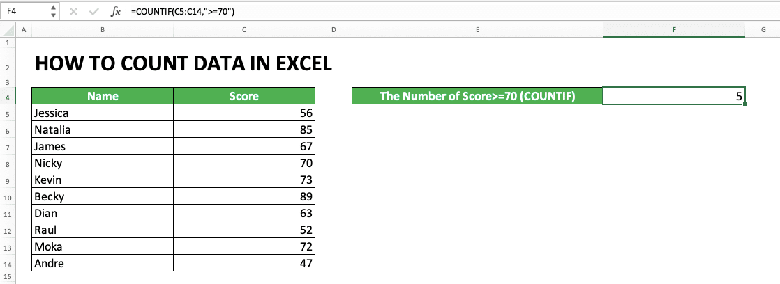
In the example, the criterion that we need to input in the COUNTIF is more than or equal to 70. The writing of this criterion input is “>=70”.

We can also see the COUNTIF writing that gives the correct counting result on the numbers that fulfill the criterion. Input the cell range and criterion correctly and you will get the right data counting result.

If you need a deeper explanation about COUNTIF, please visit this particular tutorial that discusses it.

Having more than one criterion for your data counting process? Please take a look at the next part which discusses COUNTIFS.

Count the Number of Cells With Data/Data Entries that Fulfill More Than One Criterion: COUNTIFS

COUNTIFS is a formula provided by excel if you want to count data/data entries with more than one criterion. How to write the formula in excel? Here is its general form.



In COUNTIFS, you can input more than one cell range with its criterion.

You need to, however, input the cell ranges and criteria in pairs. That means the criterion which follows a cell range in COUNTIFS will evaluate the data in that cell range only.

COUNTIFS will count the data entries which all parallel data fulfill all the criteria you input. If one of its data doesn’t, then a data entry won’t be counted. Usually, we give the cell range input per one column, with each entry in which all columns fulfill the criteria is counted.

If what you want is one cell range but with many criteria, then input the cell range repeatedly. The writing of the criterion in COUNTIFS is the same as COUNTIF. If you need to learn this, then please see the next part of this tutorial.

To make it clearer for the explanation, let’s see the example of COUNTIFS usage in excel below.



In the above example, there are three score columns. We want to count the number of people that have all three of their scores above 70. To get that result we need, we use COUNTIFS.

You can see in the COUNTIFS writing in the formula bar, how the pairing of cell ranges and criteria is done. We input the score column’s cell range one by one, followed by the score criterion after the cell range is inputted. Because, in this example, the criterion is the same (more than 70), we input “>=70” after each score column’s cell range input.

Input correctly the cell ranges and criteria pairings, then you will get the right COUNTIFS result.

If you want to learn more about COUNTIFS, please visit this tutorial which discusses it.

The Criteria Writing in COUNTIF and COUNTIFS

How to write the criterion input in COUNTIF and COUNTIFS? First, of course, you need to know the constraints you want for the data you want to count. Only after that, you try to find how to translate those constraints into criteria writing in excel.

You can learn various types and forms of criterion writing and the meaning of each below.

Text (not case-sensitive)

Criterion Example	Explanation
"Jim"	The same as “Jim”
“<>Jim”	Not the same as “Jim”
“Jim*”	With “Jim” prefix
“*jim”	With “jim” suffix
“J*m”	“J” prefix and “m” suffix
“Jim?”	“Jim” prefix with any one character suffix
“?jim”	Any one character prefix with “jim” suffix
“J?m”	“J” prefix, any one character, and “m” suffix
“Jim~*”	The same as “Jim*”
“Jim~?”	The same as “Jim?”

A bit explanation of the symbols used for the text criterion:

• * = any character with any amount
• ? = any one character
• ~ = used when you want to add * or ? character for the criterion

Number

Criterion Example	Explanation
70	Equal to 70
“>70”	More than 70
“<70”	Less than 70
“>=70”	More than or equal to 70
“<=70”	Less than or equal to 70

Date

Criterion Example	Explanation
“>”&DATE(2019,12,3)	Later than 3 December 2019

It isn’t recommended to input a date criterion with direct writing (e.g. “>3-12-2019”). This can produce a wrong and unexpected result.

Cell coordinate

Criterion Example	Explanation
“>”&B1	More than the value in B1

Empty/non-empty cell

Criterion Example	Explanation
“"	Empty
“<>"	Not empty

Count The Amount of Unique Data: SUMPRODUCT COUNTIF

After finish discussing the five data counting formulas in excel, now we talk about using formula combinations to count excel data.



Formula combinations are needed when your data counting needs cannot be fulfilled with the five formulas functions discussed previously. One of the examples of the need is if we want to count unique data in a cell range. How to do that?

You can count unique data by combining the SUMPRODUCT and COUNTIF formulas.

How to combine them to do that? Here is the general writing form.



Confused about how this formula combination works? See the example of SUMPRODUCT and COUNTIF usage below and the explanation after that.



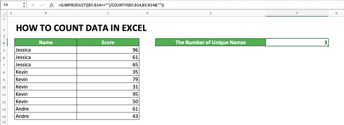
In the example, we can see how SUMPRODUCT and COUNTIF are used to count unique data in the name column. As you can see, this combination can give the amount of unique data in that column, which is 3.

We can use SUMPRODUCT to make a formula that usually accepts individual data input to accept a cell range input. In this case, SUMPRODUCT is used to help to process COUNTIF criterion input.

Here, we count each data in the name column with the data itself as the criterion. This can be done by inputting the name column’s cell range as the criterion input too. In the criterion input, we also input &”” to anticipate empty cells, if there is any.

With the COUNTIF writing like that, the result will be an array of data like this:



Can you guess what are those 3, 5, and 2 numbers represent? They represent the frequency of each data in the name column. Jessica shows up 3 times, Kevin 5, and Andre 2. Because of the array results here also that we need SUMPRODUCT to facilitate the process.

In the SUMPRODUCT input before COUNTIF, we write that each data in our cell range shouldn’t be empty data (<>””). This is also to anticipate empty cells in the cell range so the SUMPRODUCT COUNTIF doesn’t produce an error.

When each data in the name column’s cell range is conditioned to not be empty, the result becomes like this.



All results are TRUE because each cell in the name column isn’t empty (if there is an empty cell, then its value will become FALSE). Because TRUE can also be represented by 1 in excel, then the result above is the same as.



We then divide the array data result with our COUNTIF result. An array division process is done in pairs between two parallel data. Because of that, the division result becomes like this in that example.



After the division happens, the SUMPRODUCT function will sum all the numbers in the resulting array. The sum result is 3 or the same as the amount of unique data in the name column’s cell range!

You can try this SUMPRODUCT COUNTIF to count unique data in your cell range. See the result for yourself!

How to Count Data in Excel for Dates With a Specific Day/Month/Year Number: SUMPRODUCT DAY/MONTH/YEAR

Date data count is something that we sometimes need in excel. Usually, we need to count dates based on the day and/or month and/or year criteria.

How to count like that in excel? This can be done by combining SUMPRODUCT and DAY/MONTH/YEAR.

Here is the general writing form of those formulas combined to count dates in excel.



The use of DAY, MONTH, and YEAR in the writing above depends on your need. Use DAY if your dates counting criterion is a day number, MONTH if month, and YEAR if year. If you just use one of those three formulas, then you don’t need to use star symbols (*).

For the symbol between the cell_range and number_criterion in DAY/MONTH/YEAR, it also depends on your need. If, for example, you need to count the date with more than 15 days, then input: DAY(cell_range)>15. Input the right symbol so your date data count result can be as what you need it to be.

For a clearer understanding of this formula combination and its result, here is its implementation example in excel.



As you can see, the date counting criterion here is related to the month and year numbers. Because of that, we use MONTH and YEAR in our SUMPRODUCT input.

The formula process itself can be explained as follows. We use SUMPRODUCT here to process the array result from the multiplication of MONTH and YEAR. This array result is produced because our MONTH and YEAR inputs are cell ranges. The two of them usually get individual data inputs.

In MONTH, we need to input a criterion of more than or equal to 6. Meanwhile, in YEAR, we need to input a criterion of equal to 2009. We write both of them with “>=6” after the MONTH’s cell range input and “=2009” after the YEAR’s cell range input.



For MONTH, because the inputs are the date cell range followed by a criterion, the result becomes an array like this.



The content of the array is the evaluation result of each data in the join date column by the criterion. For example, for Jessica’s join date, the MONTH result is 4 (the month number of the join date). Because 4 is less than 6, the result in the array becomes FALSE for Jessica’s join date. We evaluate each data in the cell range until all the TRUE/FALSE results in the array are collected.

For YEAR, here is the array result from the evaluation of the join date’s column data by its criterion.



The evaluation process and TRUE/FALSE result principle are the same as MONTH. The criterion for the YEAR is the year number must equal 2009. Thus, the evaluation result is adjusted with this criterion.

Then, because there is a * symbol between MONTH and YEAR, both array results will be multiplied. Because TRUE is the same as 1 and FALSE is 0 in excel, then the multiplication result becomes as follows.



Arrays multiplication principle is it will multiply all data with the same position. Because of that, we get the 1 and 0 results like the one above.

And finally, because SUMPRODUCT will sum its array input, it will produce 3 from the last array. This 3 becomes the result of the date counting result with the month and year numbers criteria!

Count Filtered Data/Numbers: SUBTOTAL

What if we filter our data in excel and then we want to count the amount of the filtered data? We can use the SUBTOTAL formula for that.

The SUBTOTAL formula can be used to process filtered data in excel. There are 11 formula choices you can use on your filtered data using SUBTOTAL. Because what we discuss here is counting data, then we will use the COUNT and COUNTA choices from SUBTOTAL (if you want to know what other formulas can be used by SUBTOTAL, visit the link given above!).

Generally, to use COUNT from SUBTOTAL on filtered data, here is the writing form.



And for COUNTA, the writing is like this.



The difference, as you can see, is only in the first SUBTOTAL input, which represents the formula you want to use. The code with more than 100 amounts from both is needed when you want to ignore the cells you hide manually (not hidden by the filter). If you want to count them too, then you need to use the code with less than 100 amount.

To make the use of SUBTOTAL clearer when you count filtered data, here is its application example in excel.

Take a look at the data form before we filter it (see the table on the left).



Now, see the result after the data is filtered to show the scores from Jessica only. We use SUBTOTAL to count the number of numbers from Jessica’s scores (that means we use the COUNT formula code in the SUBTOTAL).



In the example, we use 2 as the code input in the SUBTOTAL because we want to use COUNT. If we input 102, then the result should be the same because there are no cells hidden manually here.

By using SUBTOTAL to count numbers from the filtered data, only the numbers shown by the filter will be counted. If you use a normal COUNT, then the numbers hidden by the filter will be counted too (as long as they are in the COUNT’s cell range input).

That’s why, if you need to count data or numbers in your filtered data, don’t hesitate to use SUBTOTAL!

Count the Number of Numbers with a Certain Cell/Font Color: XLTools

Want to count the number of numbers with a certain cell/font color in your data table in excel? Maybe you have marked their cells with a color code and you want to count those cells based on that code.

Unfortunately, there isn’t a built-in feature/formula provided by excel to do this kind of counting process. However, if you use XLTools, you can do it easily using one of its features!

So, how to count the number of numbers based on a certain cell/font color using XLTools? To make it clearer, please take a look at the following implementation example. Let’s say we have a score data table we have marked with colors based on its score values like below.



To count our numbers according to their colors, follow these simple steps. First, highlight the cell range you want to count the number of numbers from based on their cell/font colors. Next, go to your XLTools tab and click the Count by Color button there.



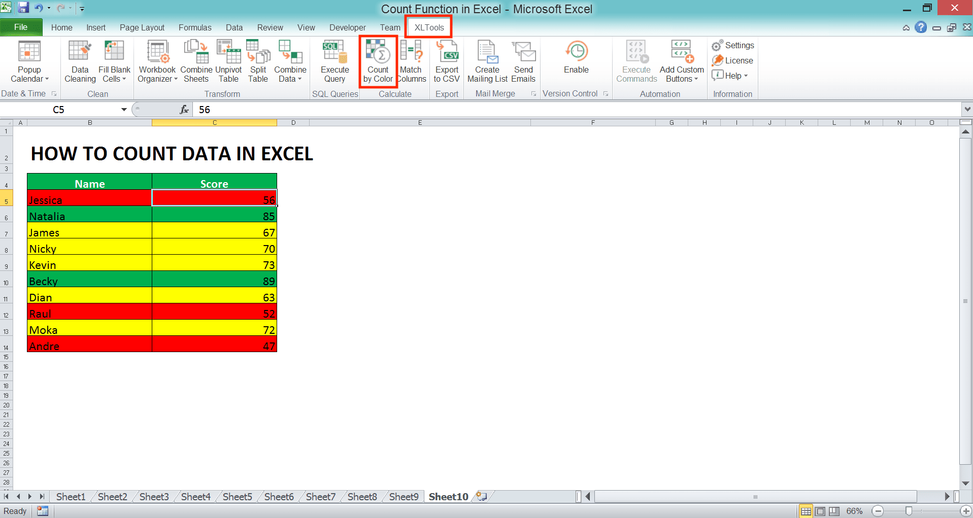
A dialog box will show itself with the cell range you highlighted that has been inputted into its text box. There are two dropdowns you can use to manage this counting process according to your preference.



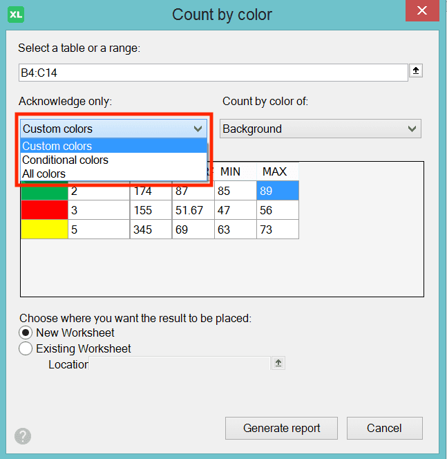
In the dropdown on the left, you can choose the color type you want to count. The choices in the dropdown with their explanation are as follow.

• Custom Colors: count your numbers based on the cell/font colors you manually give to your cells
• Conditional Colors: count your numbers based on the cell/font colors from a conditional formatting result
• All Colors: count your numbers based on the cell/font colors you manually give to your results and from the conditional formatting too

In the dropdown on the right, choose whether you want to count based on the cell color or the font color.



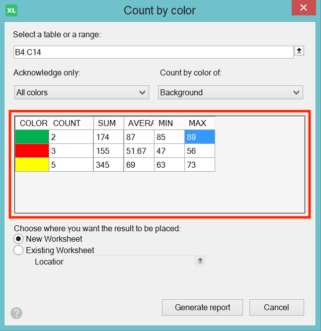
The box right below those dropdowns contains the result that you will get in your worksheet from the counting process.



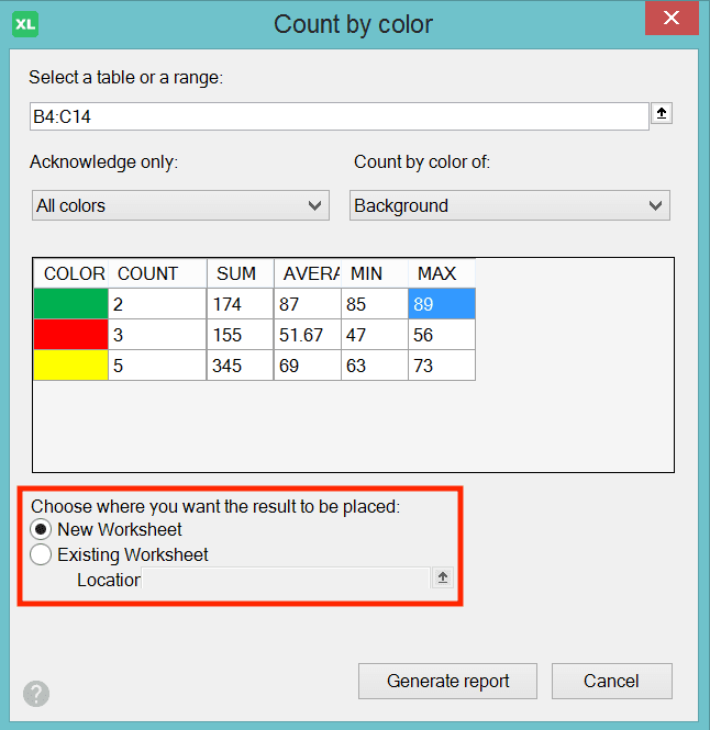
In the choices below it, you can choose where you will put the counting result in your excel file. You can choose to put it in a new worksheet (New Worksheet) or in the worksheet where your data table is (Existing Worksheet).

If you choose Existing Worksheet, then another dialog box will show up. It will help you choose the most top-left cell where XLTools will put your result.



Determine the result location and click the Generate Report button. You will get your numbers counting result based on their colors.



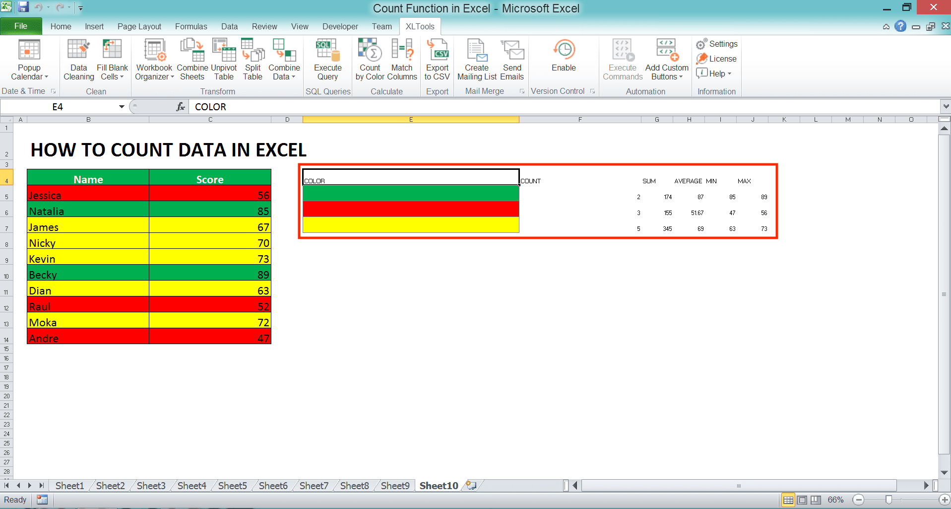
From the XLTools result, you will also get the SUM, AVERAGE, MIN, and MAX of your numbers, categorized by colors. If there are results you don’t need, just delete them.

Exercise

After you have learned how to count data in excel using various methods, now let’s do an exercise. This is so you can deepen your understanding of the learnings that have been given!

Download the exercise file and answer all the questions. Please download the answer if you have done the exercise and sure about the results!

Link to the exercise file:
Download here

Questions

1. How many filled cells are there in those four columns?
2. How many cells are empty?
3. How many data with the criteria: region 1, product C, and sold more than 100?

Link to the answer key file:
Download here

Additional Note

• COUNTA and COUNTBLANK will count all the cells contain formulas that produce empty results (“”)
• COUNTIF and COUNTIFS aren’t case-sensitive

Related tutorials you should learn: