How to Use the SUBTOTAL Formula in Excel: Functions, Examples, and Writing Steps
Home >> Excel Tutorials from Compute Expert >> Excel Formulas List >> How to Use the SUBTOTAL Formula in Excel: Functions, Examples, and Writing Steps


In this tutorial, you will learn how to use the SUBTOTAL formula/function in excel.
When working in excel, we sometimes need to process data from a cell range that has been filtered. With SUBTOTAL, you can do that much easier.
Want to know more about this SUBTOTAL function and how to use it optimally to support your work in excel? Let’s get into it.
Disclaimer: This post may contain affiliate links from which we earn commission from qualifying purchases/actions at no additional cost for you. Learn more
Want to work faster and easier in Excel? Install and use Excel add-ins! Read this article to know the best Excel add-ins to use according to us!
Table of Contents:
- What is the SUBTOTAL formula in excel?
- SUBTOTAL function in excel
- SUBTOTAL result
- Excel version from which we can start using SUBTOTAL
- The way to write it and its inputs
- SUBTOTAL function code
- Example of its usage and result
- Writing steps
- SUBTOTAL with criteria (SUBTOTAL IF)
- Apply a quick SUBTOTAL for a filtered number sequence: AutoSum
- Exercise
- Additional note
What is the SUBTOTAL Formula in Excel?
SUBTOTAL is a function you can use to process filtered data in excel.SUBTOTAL Function in Excel
You can use SUBTOTAL to get the results of some functions from the data in a filtered cell range. The functions you can apply with SUBTOTAL are AVERAGE, COUNT, COUNTA, MAX, MIN, PRODUCT, STDEV, STDEVP, SUM, VAR, and VARP.SUBTOTAL Result
The result of a SUBTOTAL formula is the processing result of filtered data with the processing type depending on your function choice in SUBTOTAL.Excel Version from Which We Can Start Using SUBTOTAL
You can use SUBTOTAL since excel 2003.The Way to Write It and its Inputs?
Here is the writing pattern of a SUBTOTAL formula in excel.
= SUBTOTAL ( function_code , filtered_cell_range1 , … )
And here is the explanation for each input needed by the SUBTOTAL formula.
- function_code = the number code that represents the function you want to apply to your filtered data
- filtered_cell_range1, … = the cell ranges of the filtered data you want to process with this function, separated by comma signs ( , )
SUBTOTAL Function Code
When writing a SUBTOTAL formula in excel, you need to input a SUBTOTAL function code as the first input of your formula. Here are the options of SUBTOTAL function codes you can input and the function that each of them represents.| Function | Calculate Cells Which Are Hidden Manually | Ignore Cells Which Are Hidden Manually |
|---|---|---|
| AVERAGE | 1 | 101 |
| COUNT | 2 | 102 |
| COUNTA | 3 | 103 |
| MAX | 4 | 104 |
| MIN | 5 | 105 |
| PRODUCT | 6 | 106 |
| STDEV | 7 | 107 |
| STDEVP | 8 | 108 |
| SUM | 9 | 109 |
| VAR | 10 | 110 |
| VARP | 11 | 111 |
As you can see above, there are two types of function codes you can use. If you want to calculate data in cells that you hide manually outside of your filtered range (not the ones that are hidden automatically by the excel filter feature or manually in your filtered range), use function codes from 1 to 11. If you want to ignore them, go with a function code from 101 to 111.
Example of Its Usage and Result
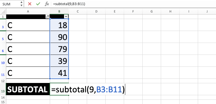
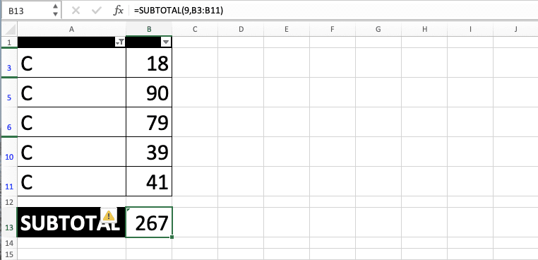
Here is an example of a SUBTOTAL implementation in excel.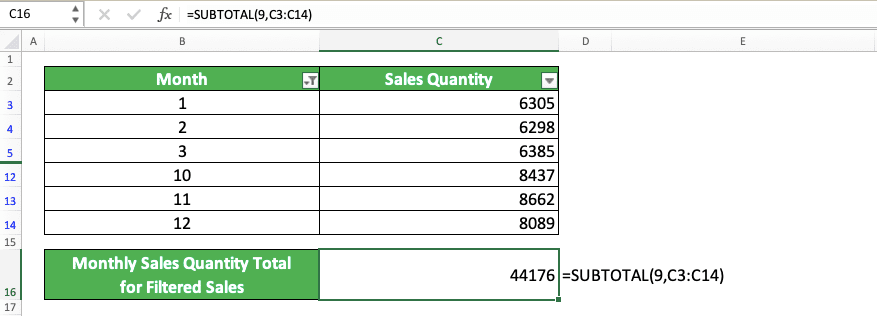
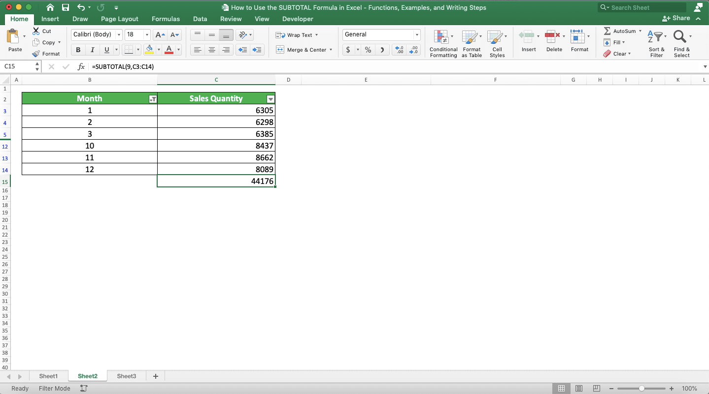
As you can see above, we use 9 as our SUBTOTAL function code there. As a result, it will apply SUM to the sales numbers in our filtered cell range. The SUM result here is 44176.
SUBTOTAL doesn’t consider the sales numbers that don’t pass our filter. As we use 9, not 109, however, it will still consider sales numbers from rows that we hide manually outside of the filtered range. However, if there are no manually hidden rows like that in our SUBTOTAL input, then we will get the same SUM result whether we use 9 or 109.
SUBTOTAL allows us to input up to 254 cell ranges in it. However, we usually only need to input one.
Writing Steps
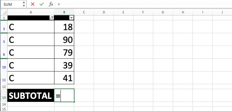
Here are the steps to write a complete SUBTOTAL formula in excel.-
Type an equal sign ( = ) in the cell where you want to put the SUBTOTAL result
-
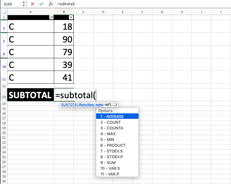
Type SUBTOTAL (can be with large letters and small letters) and an open bracket sign after =
-
Input the code of the function that you want to use (for the code reference, see the above table), after the open bracket sign. Then, type comma sign

-
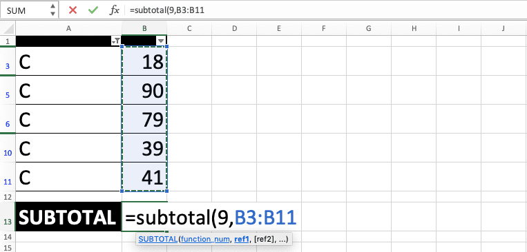
Input the filtered cell range which data you want to process with SUBTOTAL. If you want to input multiple cell ranges, separate them with comma signs
-
Type a close bracket sign
- Press Enter
-
The process is done!
SUBTOTAL with Criteria (SUBTOTAL IF)
Want to apply criteria to the filtered data you process with SUBTOTAL?Unfortunately, there is no such thing as SUBTOTALIF like SUM with its SUMIF and SUMIFS or COUNT with its COUNTIF and COUNTIFS. However, we can produce more or less the same result we want by combining SUBTOTAL with SUMPRODUCT, OFFSET, ROW, and MIN functions.
Here is the general writing format of the five functions combination to add criteria to the data processed by our SUBTOTAL.
{ = SUMPRODUCT ( ( criterion_range1 = criterion1 ) * ( criterion_range2 = criterion2 ) * … * ( SUBTOTAL ( function_num , OFFSET ( filtered_range_first_cell , ROW ( filtered_range ) - MIN ( ROW ( filtered_range ) ) , 0 ) ) ) ) }
In the combination, we use an array formula form (as you can see by looking at the curly brackets surrounding the formula) because we process arrays here. Because of that, we should press Ctrl + Shift + Enter buttons after we write the formula.
In this formula, SUMPRODUCT helps the formula to consider the criteria that we have for our filtered range. Meanwhile, the combination of OFFSET, ROW, and MIN formulas help SUBTOTAL to produce an array that can be processed with the SUMPRODUCT result to help us get the final result that we want (the SUBTOTAL result that considers data criteria)
It is important to note, though, that this formula seems to only work for the COUNT, COUNTA, and SUM functions of SUBTOTAL.
Still confused with the formula after reading that explanation? Well, take a look at the example below.
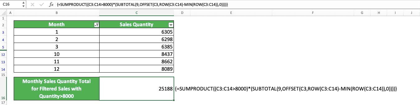
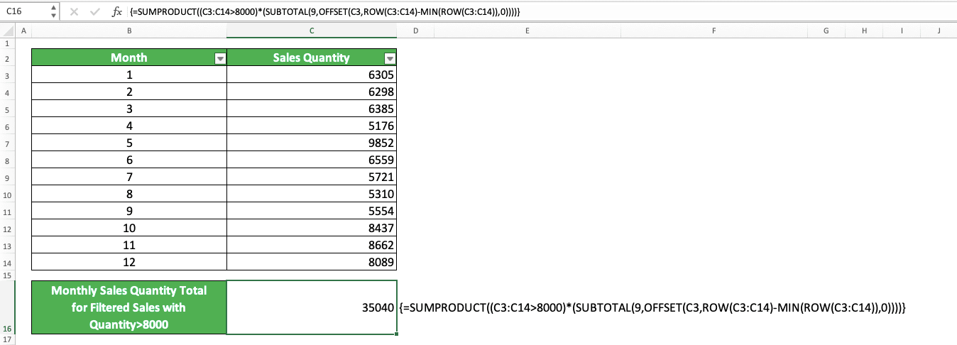
As you can see in the example, we can add a criterion to the SUM of our SUBTOTAL (sales quantity of more than 8000) by using the SUMPRODUCT, SUBTOTAL, OFFSET, ROW, and MIN functions combination. As a result of the combination, the data that doesn’t fit our criteria get ignored and we get 25188 as our SUBTOTAL result.
To understand what is going on in the formula, first, we will take a look at the first part of our SUMPRODUCT, which is the filtered range that we want to evaluate with our criterion.
As we want to filter the cell range that is processed by SUBTOTAL based on the sales quantity, we input the sales quantity column cell range here (C3:C14). We also add our criterion after the cell range input (>8000) so it can evaluate each data in the cell range.
The evaluation produces TRUEs and FALSEs. Because of this, the result of this first part of our SUMPRODUCT formula is a TRUE/FALSE array like the one below.
{ FALSE , FALSE , FALSE , FALSE , TRUE , FALSE , FALSE , FALSE , FALSE , TRUE , TRUE , TRUE }
Why there are 12 TRUE/FALSEs here instead of six like the number of sales quantities that we can see in the example screenshot? Because there are 12 sales quantities before we filter the sales quantity table as you can see below.
This also means the first part of our SUMPRODUCT formula doesn’t ignore data that has been filtered out. To help with this, we use the second part, which includes our SUBTOTAL formula, to help us.
In the SUBTOTAL formula, we use 9 as our function code as we want to sum our filtered sales quantities (we can also use 109 as we don’t input manually hidden cell ranges outside of our filtered one). As a SUBTOTAL formula produces a single result, not an array result that we need to do the multiplication with the first part of our SUMPRODUCT formula, we use an OFFSET formula to help us get an array result.
For the cell reference input of the OFFSET (the first input), we input the first cell of our filtered sales quantity column. This is because we later want our array to get the SUBTOTAL result from the first cell of the column to its last. To get OFFSET to “stretch” until the last cell of the filtered sales quantity column, we combine ROW and MIN formulas in our second OFFSET input.
In the example, our ROW(C3:C14) formula produces an array like this.
{ 3 , 4 , 5 , 6 , 7 , 8 , 9 , 10 , 11 , 12 , 13 , 14 }
That is the row numbers of all of the cells in our filtered sales quantity column. As for our MIN(ROW(C3:C14)) formula, it produces this array.
{ 3 , 3 , 3 , 3 , 3 , 3 , 3 , 3 , 3 , 3 , 3 , 3 , 3 }
Why do we need these 12 threes array from our MIN and ROW combination? That is because we want to subtract the previous array produced by our ROW with it so we can get the right array to “stretch” our first sales quantity cell by using OFFSET.
The result of the two arrays’ subtraction is something like this.
{ 0 , 1 , 2 , 3 , 4 , 5 , 6 , 7 , 8 , 9 , 10 , 11 }
It makes our OFFSET moves our first sales quantity cell multiple times according to the array numbers. The result is something like this.
{ C3 , C4 , C5 , C6 , C7 , C8 , C9 , C10 , C11 , C12 , C13 , C14 }
As our SUBTOTAL does its operation for each of the array members, it produces something like this.
{ 6305 , 6298 , 6385 , 0 , 0 , 0 , 0 , 0 , 0 , 8437 , 8662 , 8069 }
The zeroes there are because SUBTOTAL ignores hidden cells in our filtered sales quantity column.
All that is left after this is to multiply the result from the first part of our SUMPRODUCT with this second part result. As TRUE is the same as 1 and FALSE is the same as 0 in excel, the multiplication result becomes an array like this.
{ 0 , 0 , 0 , 0 , 0 , 0 , 0 , 0 , 0 , 8437 , 8662 , 8069 }
After summed by SUMPRODUCT, it will become the sales quantity total that we want to calculate here (sales quantity total for the filtered quantity above 8000), which is 25188!
Apply a Quick SUBTOTAL Sum for a Filtered Number Sequence: AutoSum
Need to sum a sequence of filtered numbers fast by using SUBTOTAL? To do that, you can use the AutoSum feature in excel.AutoSum is a feature that can help us to produce a SUM formula to sum a sequence of numbers fast by just clicking a button or pressing its shortcut buttons. If it detects that the sequence of numbers you want to sum is in a filtered range, it will produce a SUBTOTAL formula instead.
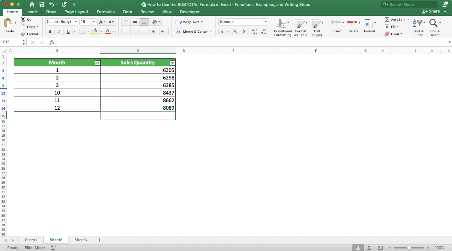
To use AutoSum to produce a quick SUBTOTAL formula, select the cell just after the number sequence in your filtered cell range like this.
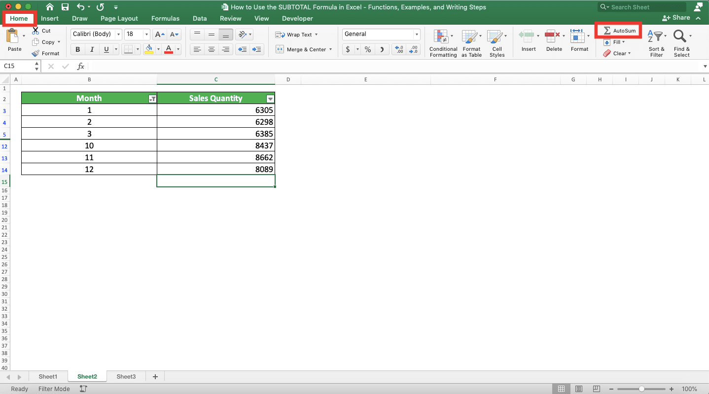
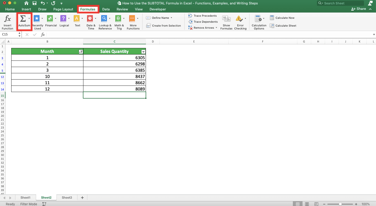
Then, go to the Home or Formulas tab of your excel ribbon and click the AutoSum button. Alternatively, you can just press Alt and = buttons simultaneously on your keyboard (Command + Shift + T for Mac).
By doing that, a SUBTOTAL formula that sums your filtered numbers will be automatically created!
Exercise
After you have learned how to use the SUBTOTAL formula in excel, you can practice your understanding by doing this exercise below!Download the exercise file from the following link and answer the questions. Download the answer key file if you have done answering all the questions and want to check your answers!
Link to the exercise file:
Download here
Questions
- What is the maximum value in column C if column A consists of letter A and column B consists of letter A or B?
- What is the average of column C values if column A consists of letter A and column B consists of letter A or B?
- What is the total of column C values if column A consists of letter A and column B consists of letter A or B?
Link to the answer key file:
Download here
Additional Notes
- SUBTOTAL ignores other SUBTOTAL results in the filtered cell range
- SUBTOTAL is designed to work on vertically arranged data. If the data is arranged horizontally, then the hidden cells will always be considered in its formula process
Related tutorials you should learn too: