Excel Cell Definition, Functions, and How to Use

In this tutorial, you will learn the excel cell definition, functions, and how to use. Cell is one of the most important excel components that you must master if you want to use excel optimally.

Disclaimer: This post may contain affiliate links from which we earn commission from qualifying purchases/actions at no additional cost for you. Learn more

Want to work faster and easier in Excel? Install and use Excel add-ins! Read this article to know the best Excel add-ins to use according to us!

Excel Cell Definition is…

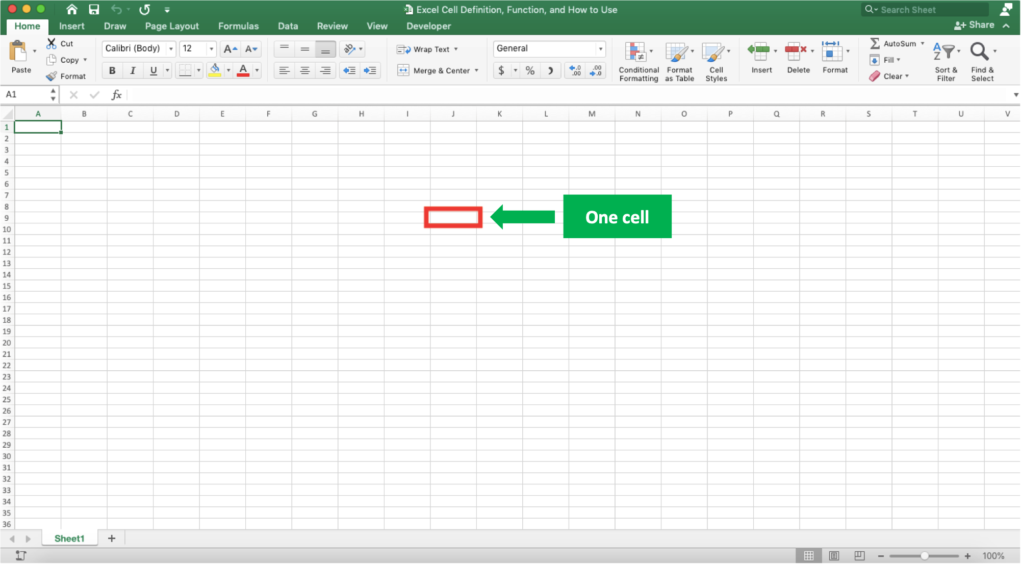
What do you mean by a cell in excel?

A cell is an intersection between a row and a column in excel. The intersection creates a place where you can input or process your data in excel.

You can see the look of what is called as an excel cell in the screenshot below.

Cell Functions

The functions of a cell in excel, among others, are:

• Becomes the place to input data in excel
• Becomes the place to process data in excel (by using formulas)
• Becomes the location reference of data which then you can use as a data reference in a formula

Cells are a crucial component in whatever the work we have in excel. By using it optimally, we can separate our data and data processing easily and clearly.

How to Select Cells in Excel

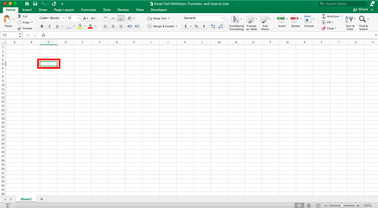
The way to select/highlight cells in excel is pretty easy.

You just need to click the cell you want to select/highlight in your worksheet. The cell you select/highlight will be marked with a green lines box around it as seen in the example below.

How to Input in Cells in Excel

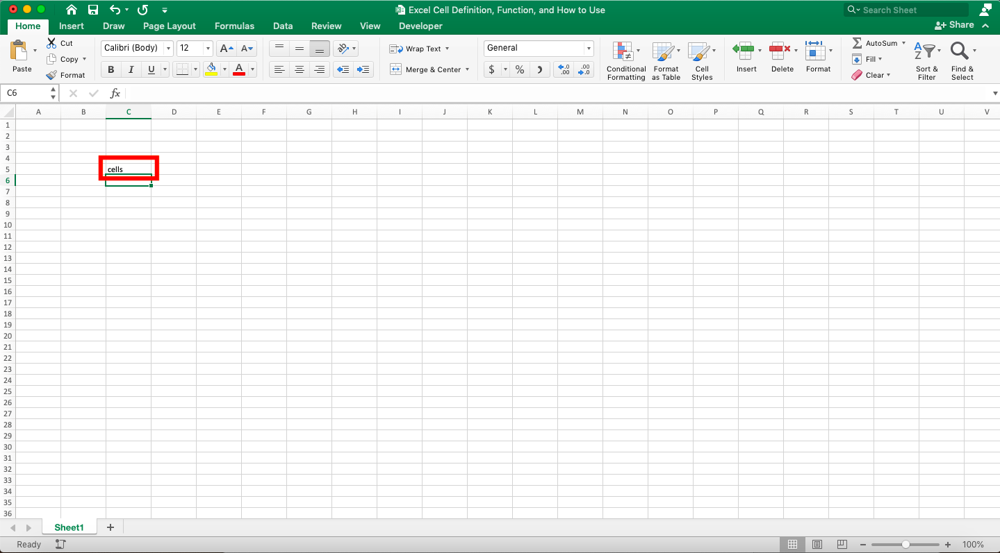
To fill an empty excel cell with data, just select the cell and type the data directly. You will automatically go to the input mode of the cell like this.



After inputting the cell, press a navigational button/click another cell/press enter. The data you type has been saved into that cell!

How to Edit Cells in Excel

What if the cell already has data and you want to edit it?

It is quite easy. If you want to delete your cell content first before retyping the data, then select the cell and directly type. Excel will automatically delete the cell data and replace it with the data you type.

If you want to edit just parts of the cell content (not all of it), then do this. Highlight the cell where the data is and then click in the excel formula bar.

The formula bar is an Excel feature that can help you to input data in excel. You can look at the display and location of a formula bar in excel in the screenshot below.



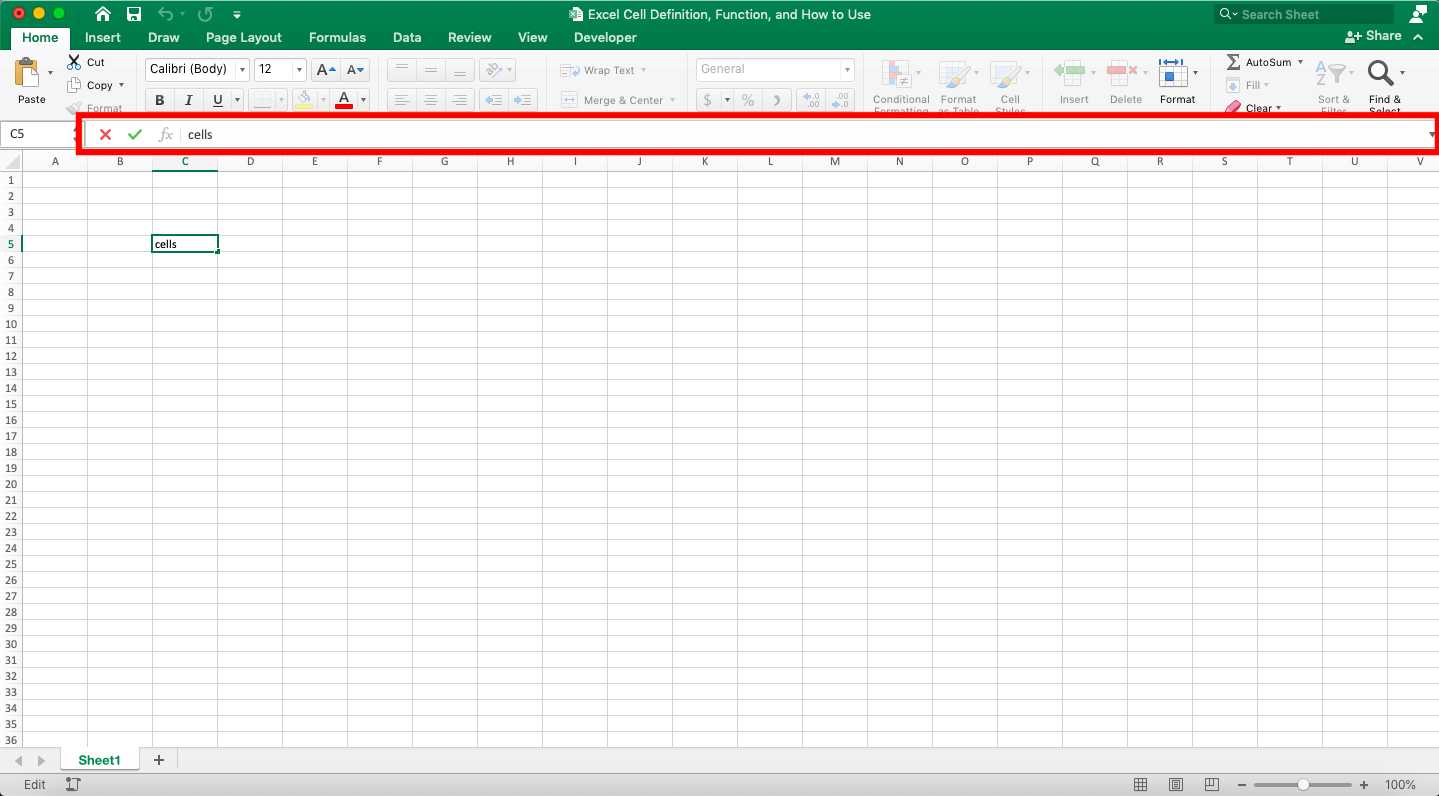
You can click the checkmark symbol in the formula bar if you have done editing the cell data. You can also click the cross symbol if you want to cancel your data editing process. Excel will return the cell data to just before you begin editing the cell if you click the cross symbol.

If you don’t want to use a formula bar, then you can also double-click the cell you want to edit. You will immediately go to the cell’s edit mode, with the cell content is still there for you to edit.

How to Delete Cells in Excel

There are two ways to delete the content of a cell in excel. The first one deletes just the content and the second deletes the content and the cell too.

As a simple example for the explanation, imagine an excel file with data like this in one of its worksheet.



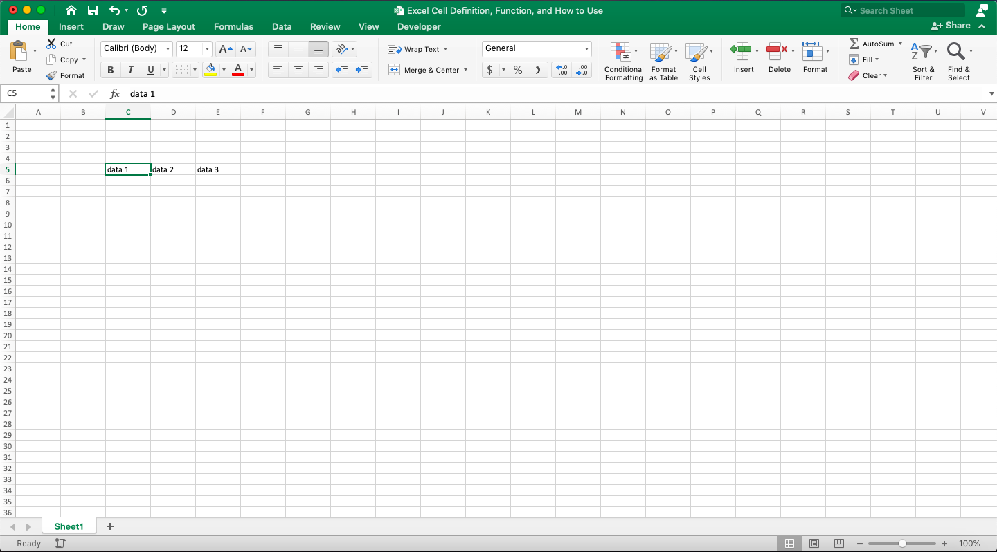
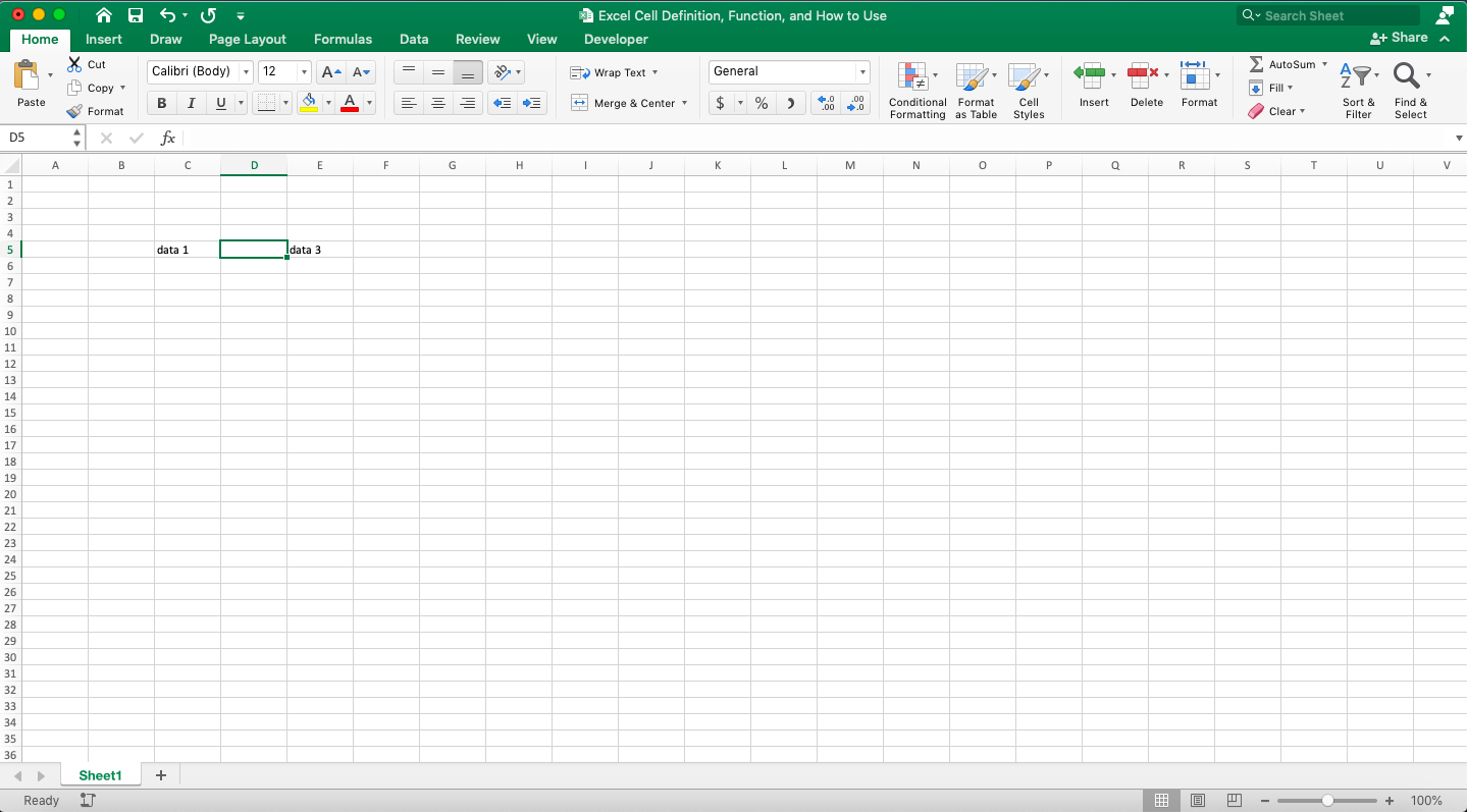
What if we want to delete the cell with the “data 2” content? If you want to just delete the cell content, then highlight the cell and press Backspace or Delete. The result will become like this.



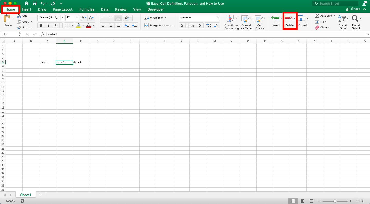
But if you want to delete the content with the cell too, then do this. Highlight the cell and click the Delete button in the Home tab of your excel. You can see the button’s exact location in excel below.



The result by using the Delete button will become like this.



See the difference? In the first result, we just delete the content while in the second result, we delete the cell too.

The first deletion method won’t cause the data in another cell to move. On the other hand, the second method causes data on the right to move one step to the left!

Why does that happen? That is because, in the second method, the deleted cell is no longer there. Thus, the data in the cell on the right moves to the left to fill the space.

How to Navigate Between Cells in Excel

If you want to move to another cell normally, just use the navigational buttons on your keyboard or click your mouse.



Or, you might want to use some shortcuts to move to a particular cell in your worksheet fast? Here are some good ones for that purpose.

Description	Windows	Mac
Move one screen to the right	Alt + Page Down	Fn + Option + ↓
Move one screen to the left	Alt + Page Up	Fn + Option + ↑
Move one screen down	Page Down	Fn + ↓
Move one screen up	Page Up	Fn + ↑
Move to the data region’s far right	Ctrl + →	Command + →
Move to the data region’s far left	Ctrl + ←	Command + ←
Move to the data region’s bottom	Ctrl + ↓	Command + ↓
Move to the data region’s top	Ctrl + ↑	Command + ↑
Move to the beginning of the row	Home	Fn + ←
Move to the most top left cell in the worksheet where the row has data	Ctrl + End	Fn + Control + ←
Move to the most bottom right cell in the worksheet where the row has data	Ctrl + Home	Fn + Control + →
Toggle End Mode	End	Fn + →
Move back to the hyperlink	Ctrl + G + Enter	Control + G + Enter

How to Copy Cells in Excel

What if we want to copy a cell’s content to another cell?

The way to do this copy process in excel is quite easy. First, you select the cell you want to copy the content from. Then, right-click and choose Copy or press the Ctrl + C shortcut (Command + C in Mac).



There will be a box with moving dotted lines that appear around the cell you want to copy. This is a mark from excel for the cell that becomes a copy source.



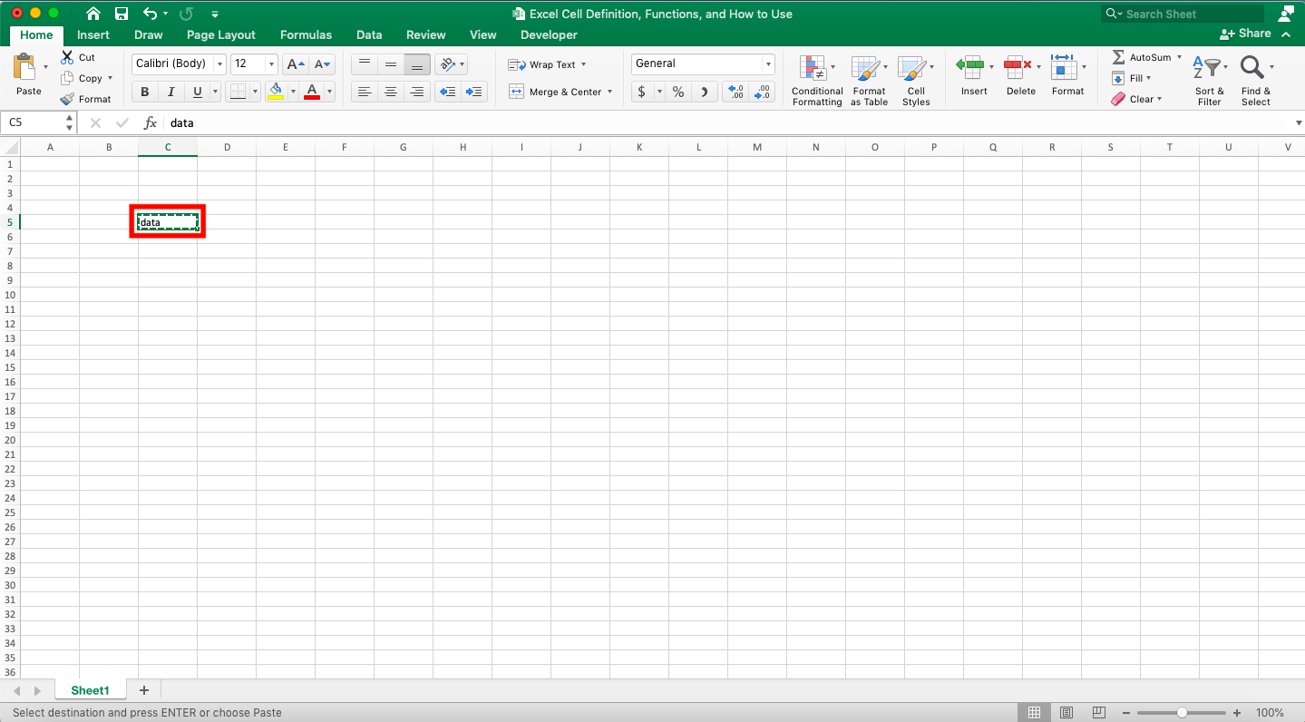
For the next step, select the cell where you want to put the copy result. Then, right-click and choose Paste or press the Ctrl + V shortcut (Command + V in Mac).



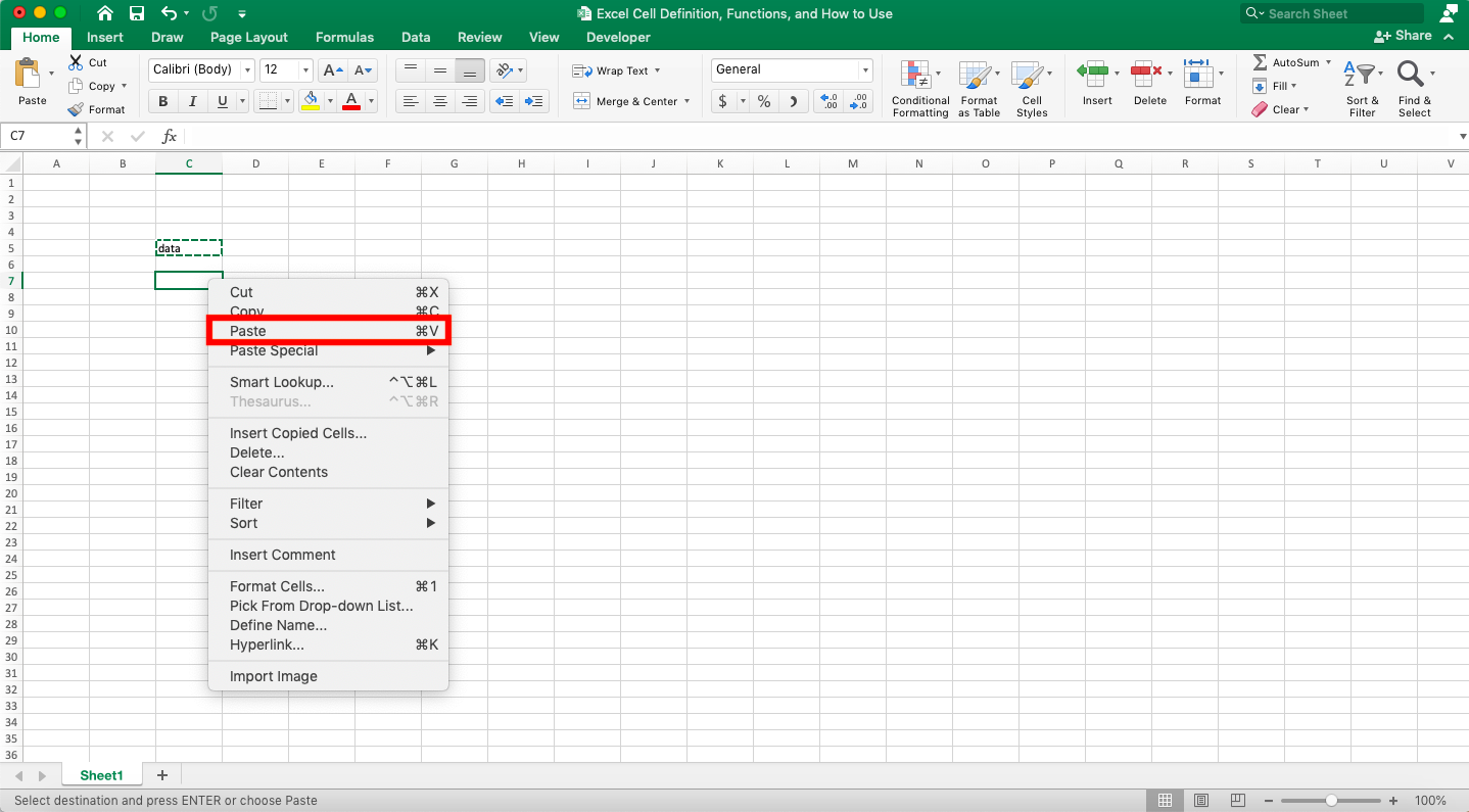
The copy process is done!



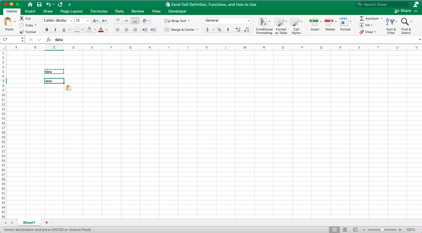
If you have copied your cell content and want to make the dotted lines around your cell disappear, press Esc. You can also input or edit a cell content to make those lines disappear.

How to Protect Cells in Excel

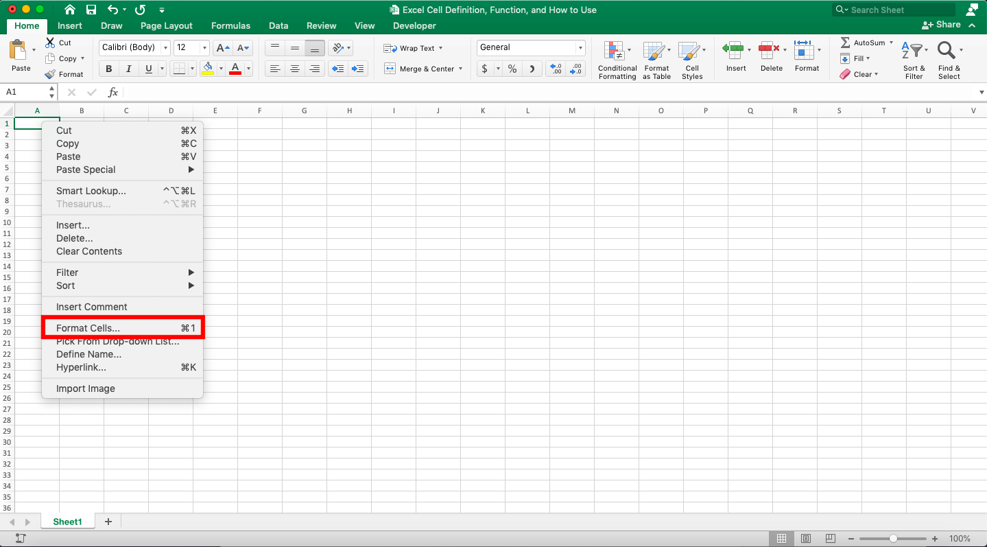
When you protect a sheet, you also automatically protect all the cells in it. But, if you only want to protect some cells, you can set that before you protect their sheet.

The way to set it is by highlighting the cells you don’t want to protect and then right-click on them. Then, choose Format Cells…



In the dialog box that appears, go to the Protection tab. Next, uncheck the Locked check box there by clicking on it, Then, click OK.



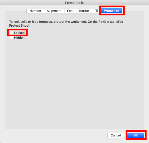
Those cells won’t be protected when you protect your sheet! The cells you don’t change the lock settings of will automatically be protected when you protect your sheet.

If you need to set the previously unlocked cells to become locked again, just check their Locked checkboxes again.

After finish managing the lock settings in your sheet, right-click on the sheet name in the bottom left. Then, choose Protect Sheet…



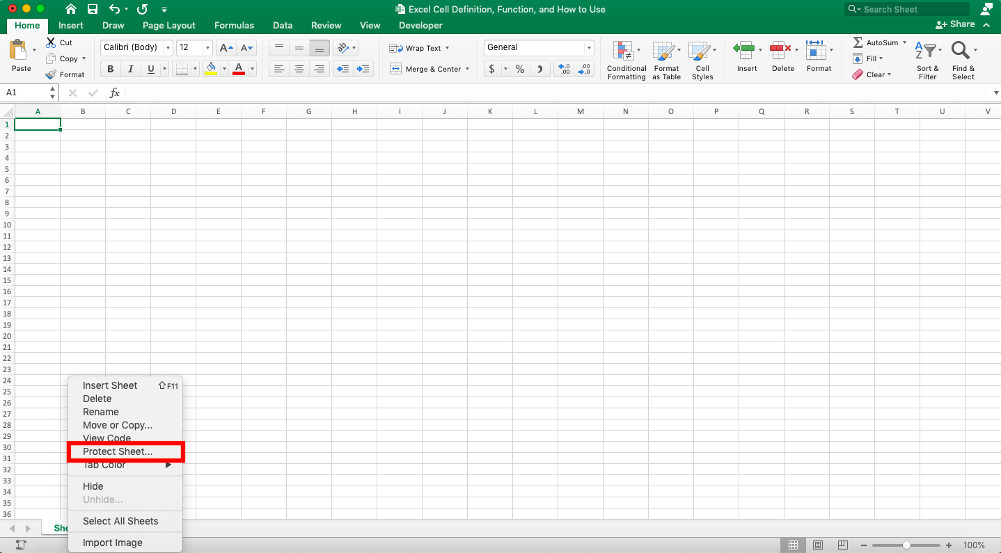
The Protect Sheet dialog box will appear.



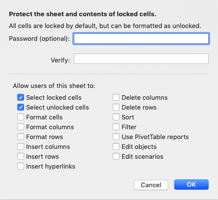
If you want, you can input a password for the sheet protection inside the text boxes of the dialog box. Excel will ask for the password if you want to unprotect the sheet.

You can also set the protection detail through the checkboxes available. Set the things allowable and unallowable when the sheet is protected there.

After determining the password and configuring the sheet protection detail, click OK.

You have protected your sheet! The cells with the checked Locked check box will be protected while the unchecked ones will be not.

How to Unprotect Cells in Excel

If to protect your cells you must protect your sheet, then to unprotect your cells you must unprotect the sheet too.

The way to unprotect a sheet is not so hard. Right-click on the protected sheet name and choose Unprotect Sheet…



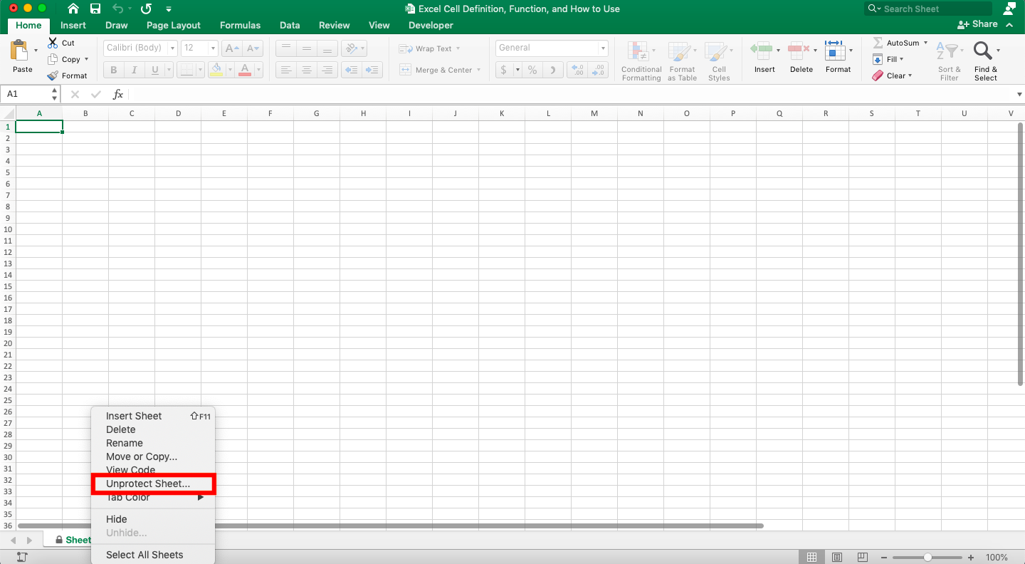
If you don’t use a password when protecting the sheet, then excel will immediately unprotect the sheet. If you use a password, then excel will ask for the password through a dialog box like this.



Input the password in the text boxes and click OK.

Your sheet will become unlocked! In that sheet, your cells that were locked will also become unlocked as a result.

Additional Note

There is a trick in excel you can use to hide your cell content! The way to do this trick is by, first, right-clicking on the cell which content you want to hide. Then, choose Format Cells…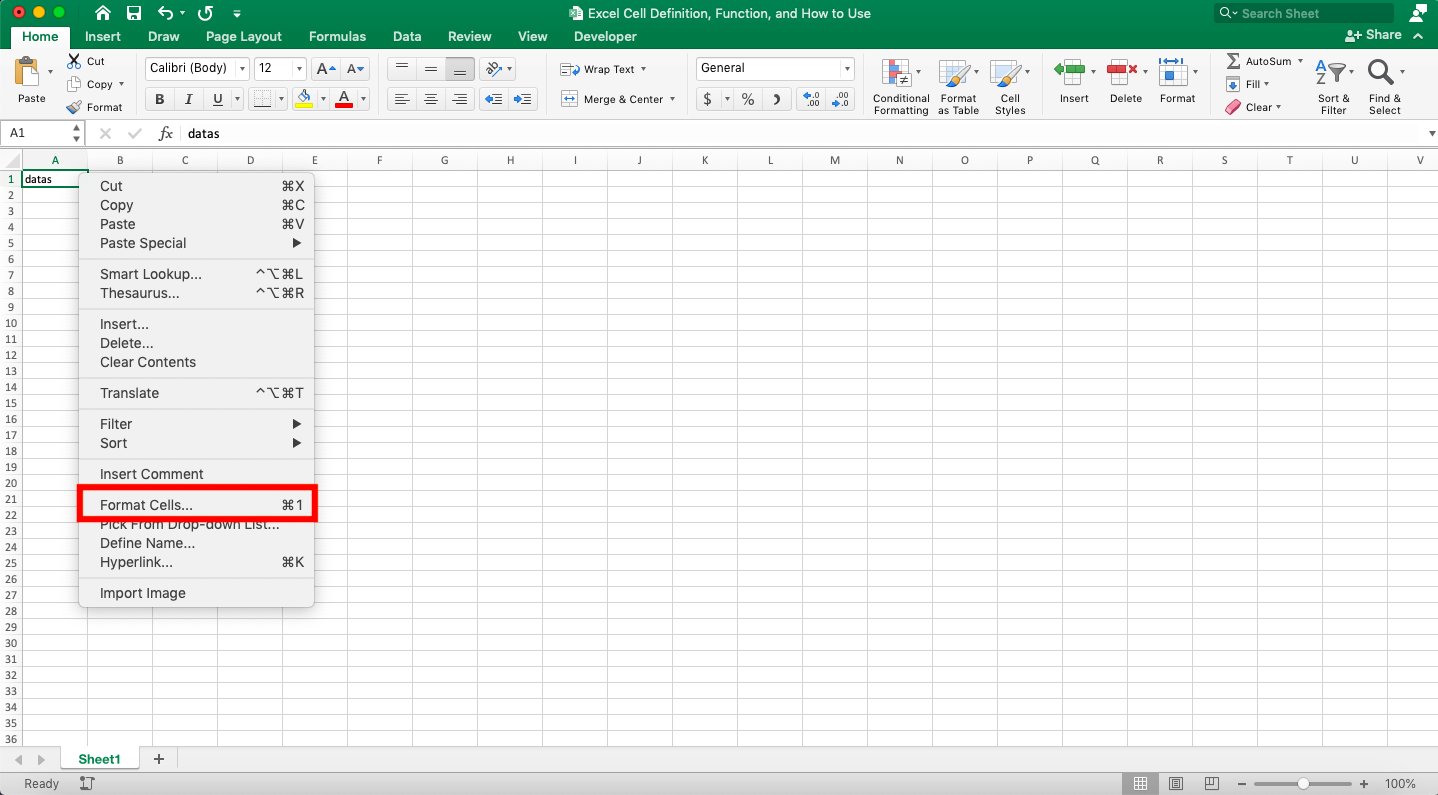



Go to the Number tab in the dialog box shown and click the Custom category. In the text box shown on the right after you choose the Custom category, input ;;;.



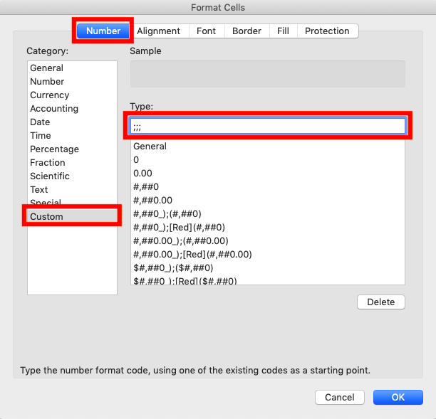
After that, click OK.

Your cell content becomes hidden! You can still see that cell content in the formula bar when you select the cell. However, the cell content won’t appear when you look at the cell in your worksheet.



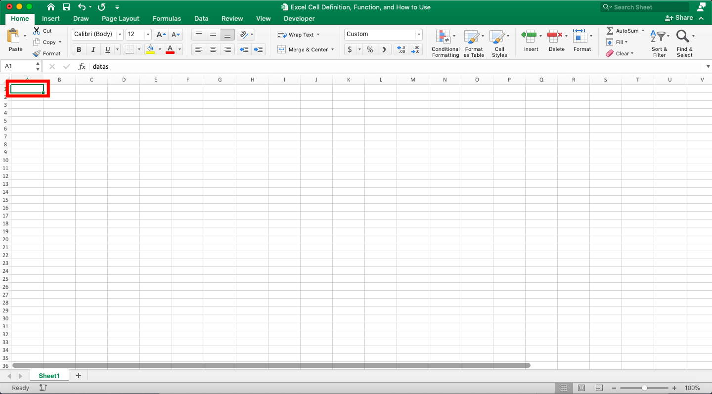
If you want to unhide the cell content, just go to the Format Cells dialog box again. Then, choose the General category in the Number tab or other categories. Last but not least, click OK to show your cell content again.



Related tutorials you should learn: