How to Sum in Excel and All Its Formulas/Functions
Home >> Excel Tutorials from Compute Expert >> Excel Calculations >> How to Sum in Excel and All Its Formulas/Functions


In this tutorial, we will learn how to sum in excel completely.
There are various methods available in excel to sum depending on our needs. Excel also has special formulas for the sum process such as SUM, SUMIF, and SUMIFS.
After reading and understanding all the contents here, you should have no problem to do a sum process in excel. You will also understand what are excel sum formulas you can use to process your data. Thus, without further ado, let’s follow all the tutorial parts until the end!
Disclaimer: This post may contain affiliate links from which we earn commission from qualifying purchases/actions at no additional cost for you. Learn more
Want to work faster and easier in Excel? Install and use Excel add-ins! Read this article to know the best Excel add-ins to use according to us!
Table of Contents:
- How to sum in excel using a manual formula writing
- How to sum in excel using the SUM formula
- How to sum in excel using click + drag
- How to sum columns in excel/to the side
- How to sum down in excel
- How to sum between sheets in excel
- How to sum time in excel
- How to sum in excel using 1 criterion: SUMIF
- How to sum in excel using more than 1 criterion: SUMIFS
- How to sum in excel for filtered data: SUBTOTAL
- How to sum in excel by ignoring errors: SUM IFERROR
- How to sum much faster in excel: AutoSum
- Exercise
- Additional note
How to Sum in Excel Using a Manual Formula Writing
The first method to sum in excel that we will discuss is by using manual sum formula writing. To do the writing, we use the plus symbol ( + ).How to write the sum formula manually in excel? Here is the general writing form.
=number_1 + number_2 + …
Pretty simple, isn’t it? The writing form is like when you write a standard sum formula everywhere, not just in excel.
Input all numbers/cell coordinates filled with numbers you want to add with + symbols between them. Don’t forget to write an equal symbol ( = ) in front of the writing as a formula writing symbol in excel.
As an example of the implementation of this writing form to sum in excel, see below.
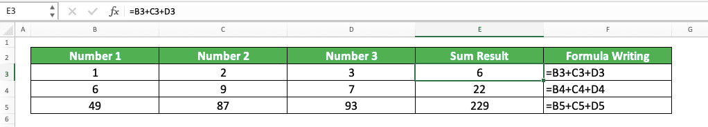
The numbers we want to sum in the example are spread into several cells. We input the cell coordinates of the numbers we want to sum and the + symbols to get the sum result.
After we have written the formula, press enter. You will immediately get your numbers sum result.
How to Sum in Excel Using the SUM Formula
If you want to use an excel formula to help your numbers sum process, then you can use SUM. This formula usage is pretty easy because you only need to input all the numbers you want to sum inside it.Generally, the SUM formula’s writing form in excel is as follows.
=SUM(number1, [number2], …)
You can input all the numbers you want to sum as needed in SUM. Usually, the input form of SUM itself is a cell range, where the numbers you want to sum are all there.
If you input more than one number/cell coordinate/cell range, don’t forget to add comma signs between your inputs.
To make it clearer about this SUM formula, here is its implementation example in excel.

In the example, we use the same numbers that we use in the manual sum formula writing example before. The sum results we get from the manual formula writing and the SUM methods are similar.
For the example, the SUM method is probably easier because we just need to input the cell range of the numbers. This is because the numbers we want to sum are near each other.
Input all the numbers you want to sum in SUM and enter. You will immediately get your numbers sum result!
How to Sum in Excel Using Click + Drag
If you don’t need your sum result in a cell (you just want to know the sum result), then there is a very fast method to get it.Just highlight all the cells which contain the numbers you want to sum. Click and drag on all the cells. Then, look at the bottom right of your excel file.
There will be the numbers sum result shows up like this (the one in the red box).
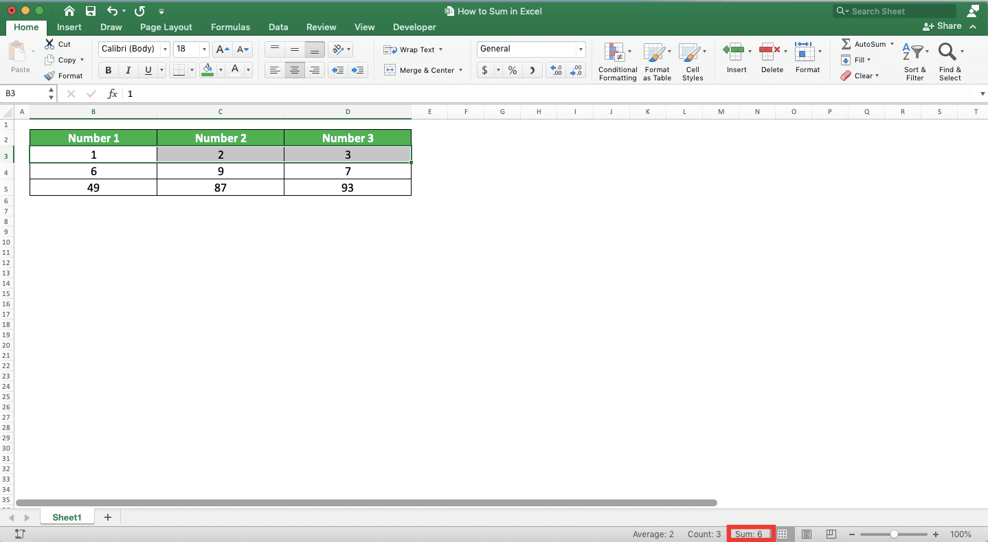
By using this method, you can get the sum result of your numbers fast!
How to Sum Columns in Excel/to the Side
Want to sum to the side, per column, to several columns you have in your excel data table? If the columns are parallel, close, and in the same size (like most columns in a data table), then use SUM and a formula copy process.As an example, take a look at the following data table.
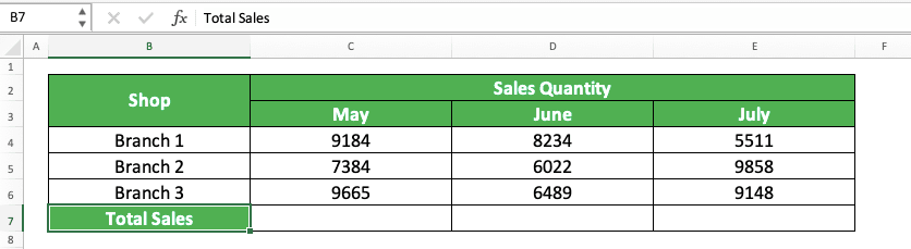
We want to get the total sales quantity per month for each store. How to do this sum process fast and accurately in excel?
First, you sum the numbers in the most left column by using a formula. You can write a sum formula manually with the + symbol or use SUM.
Because the numbers we want to sum are in a cell range, it is probably easier if we use SUM.
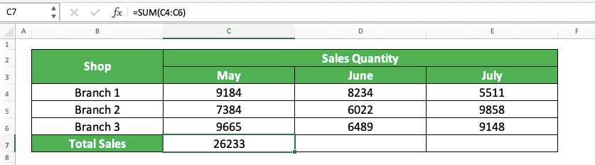
Don’t forget to add the numbers in their cell coordinates form, not by typing them directly. This is so we can easily copy the formula later to the side to get other columns’ sum results.
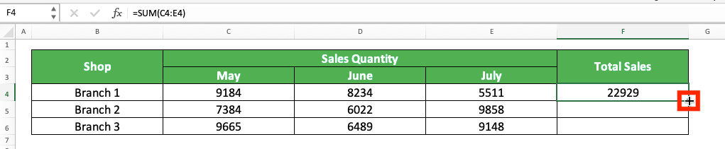
After done writing the sum formula for one column, we copy the formula to the right. The way to copy it is by first highlighting the cells where your sum formula is. Then, move the pointer to the bottom right of the cell cursor (to the little box on the cell cursor) until it becomes a + symbol like this.
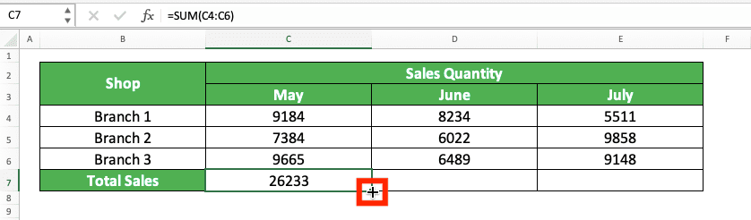
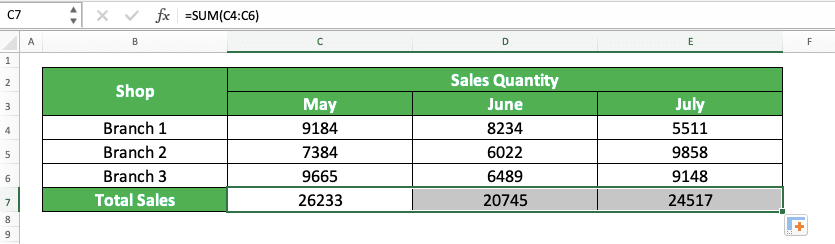
After your pointer becomes a +, click and drag to the right until the last column that you want to sum. When you get to the last column, release your drag. You will get the sum results of the columns in your data table!
That is how you sum columns in excel. If you understand how to copy a formula in excel, then you should get your sum results quickly.
How to Sum Down in Excel
What if what we want to sum is numbers per row or down as per its direction? The method is pretty similar to the columns sum method earlier.To make this clearer, look at the data table we use for the columns sum process earlier.
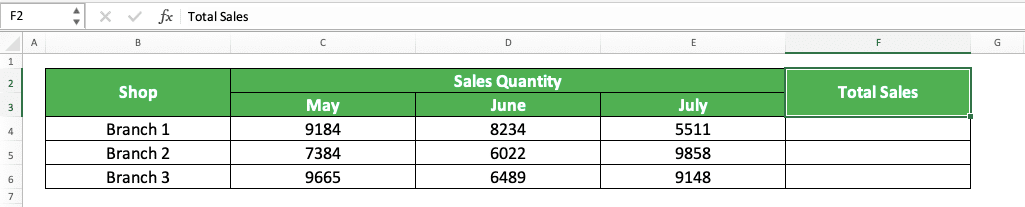
Now, we want to get the total sales quantity per shop branch. How to do that?
Similar to the sum process of the columns earlier, we write the sum formula for the first row numbers first.
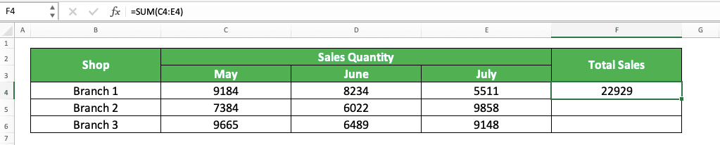
After we get the sum result of the first row, we highlight the cell with the sum formula. Move our pointer to the bottom right of the cell cursor until it becomes a + symbol like this.
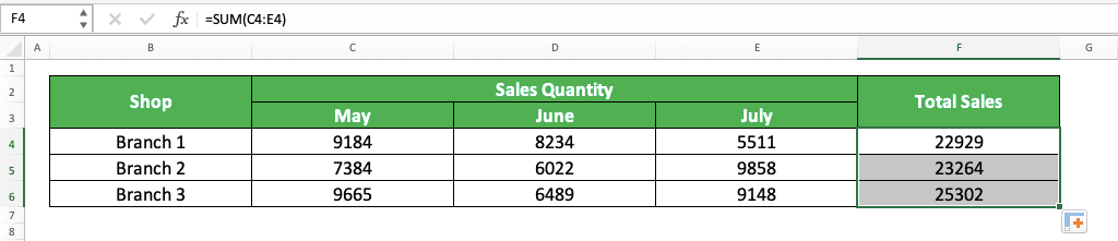
Click and drag our pointer until the last row that we want to get the numbers sum result from. Release the drag after we reach that last row. We will immediately get all the rows sum results we want!
Similar to the columns sum process before, right? You must know how to copy a formula in excel so you can get your sum results fast and accurately.
How to Sum Between Sheets in Excel
Sometimes, maybe the numbers we want to sum are in different sheets to where we want to put our sum result. What should we do in this situation?Fortunately, Excel makes it easy to refer to numbers in different worksheets. Just input the sheet name before we input the cell coordinate where the number is in our sum formula. We do the sum process with this approach.
We can use the sum formula we write manually or SUM for this. Generally, the writing forms for each method for this different sheets’ sum process are as follows.
Manual sum formula writing:
=‘sheet_name’number_cell_1 + ‘sheet_name’number_cell_2 + …
SUM:
=SUM(‘sheet_name’number_cell_1 , [‘sheet_name’number_cell_2] , …)
When inputting the cell containing the number, you can go to the sheet where the cell is and click the cell. By doing that, the sheet name and the cell coordinate will automatically be inputted into your formula. You don’t have to write them on your own.
To understand better about this sum process, see the example below.

Here, we want to sum numbers from the June and July sheets, which contain data like these.

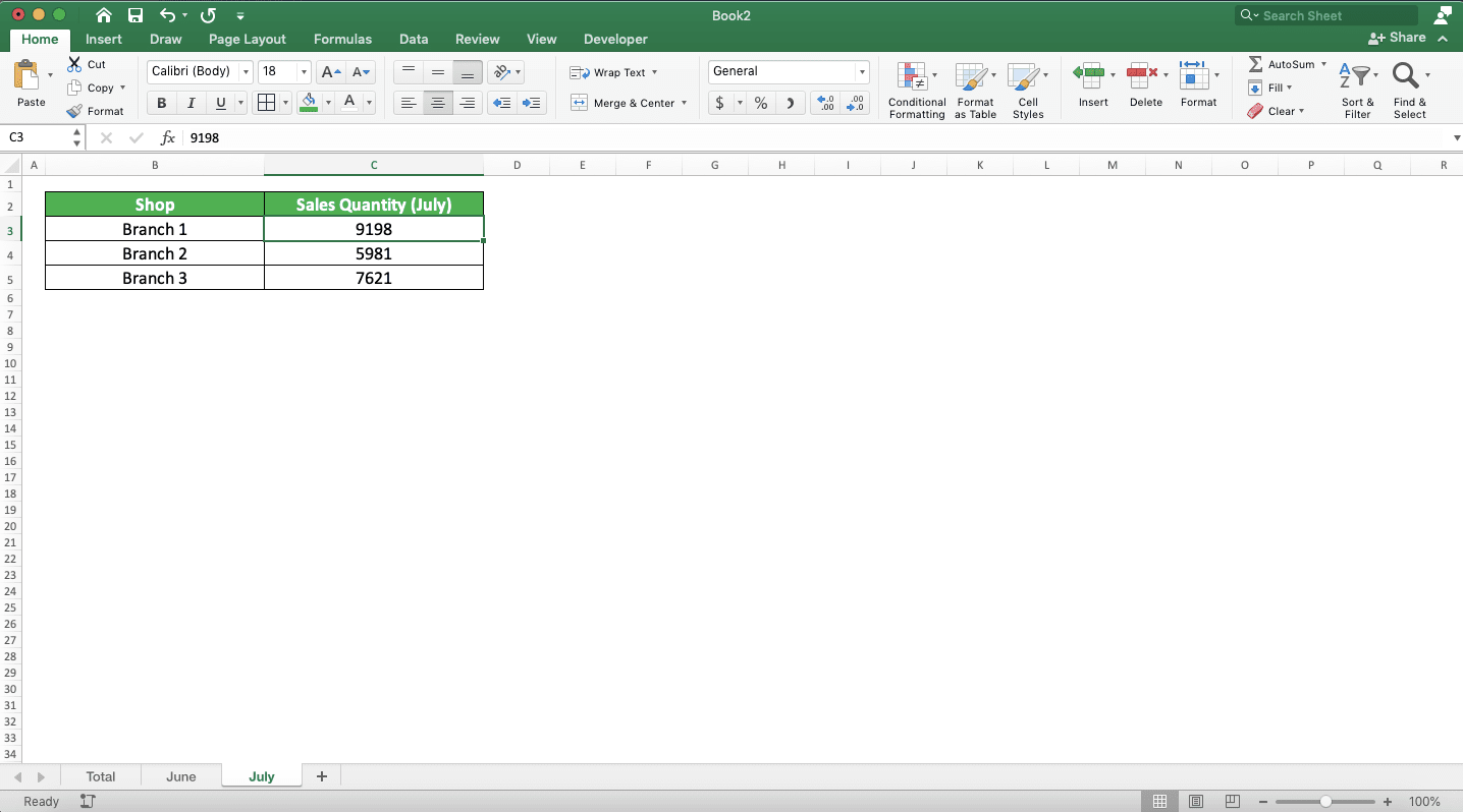
How to do the sum in the “Total” sheet of the example excel file?
First, we type the = symbol in the place where we want to put the sum result as usual.
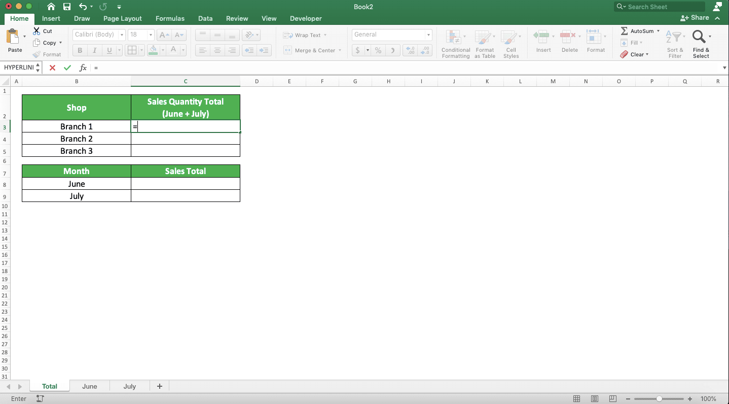
For manual sum formula writing, we can directly get the number from another sheet to sum it. We do that by going to the sheet where the number is and click the cell containing the number like this.
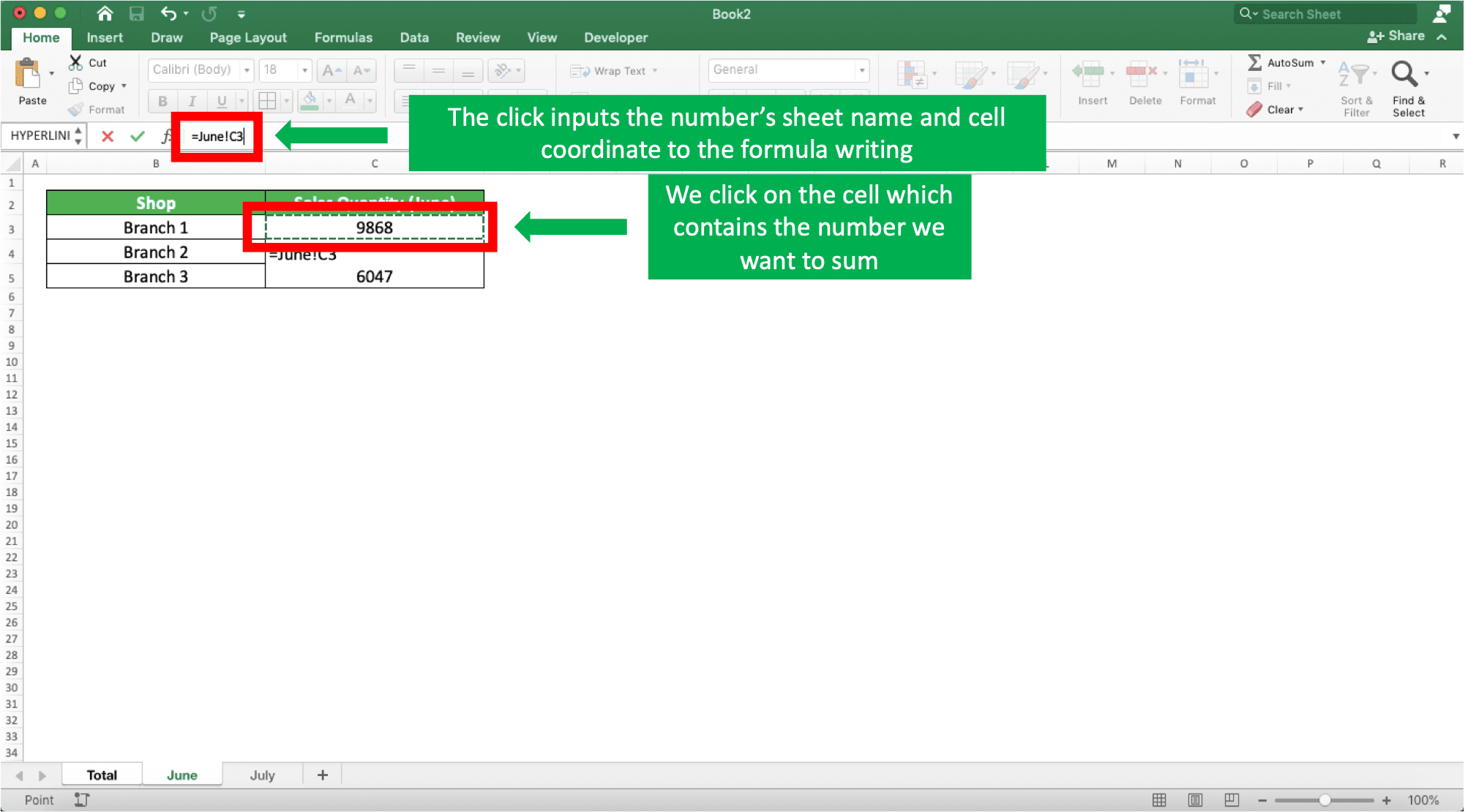
Do that for all the numbers we want to sum while we type our sum formula. After all the numbers are inputted, press enter. You will immediately get the sum result!
What if we want to use SUM to get the different sheets sum result? The approach is almost the same.
First, we type the SUM until the part where we need to input the numbers.

Then, we go to another sheet and input the numbers to sum by clicking the cell/dragging the cell range. Because all the numbers we want to sum in the example are in a cell range, we input like this.
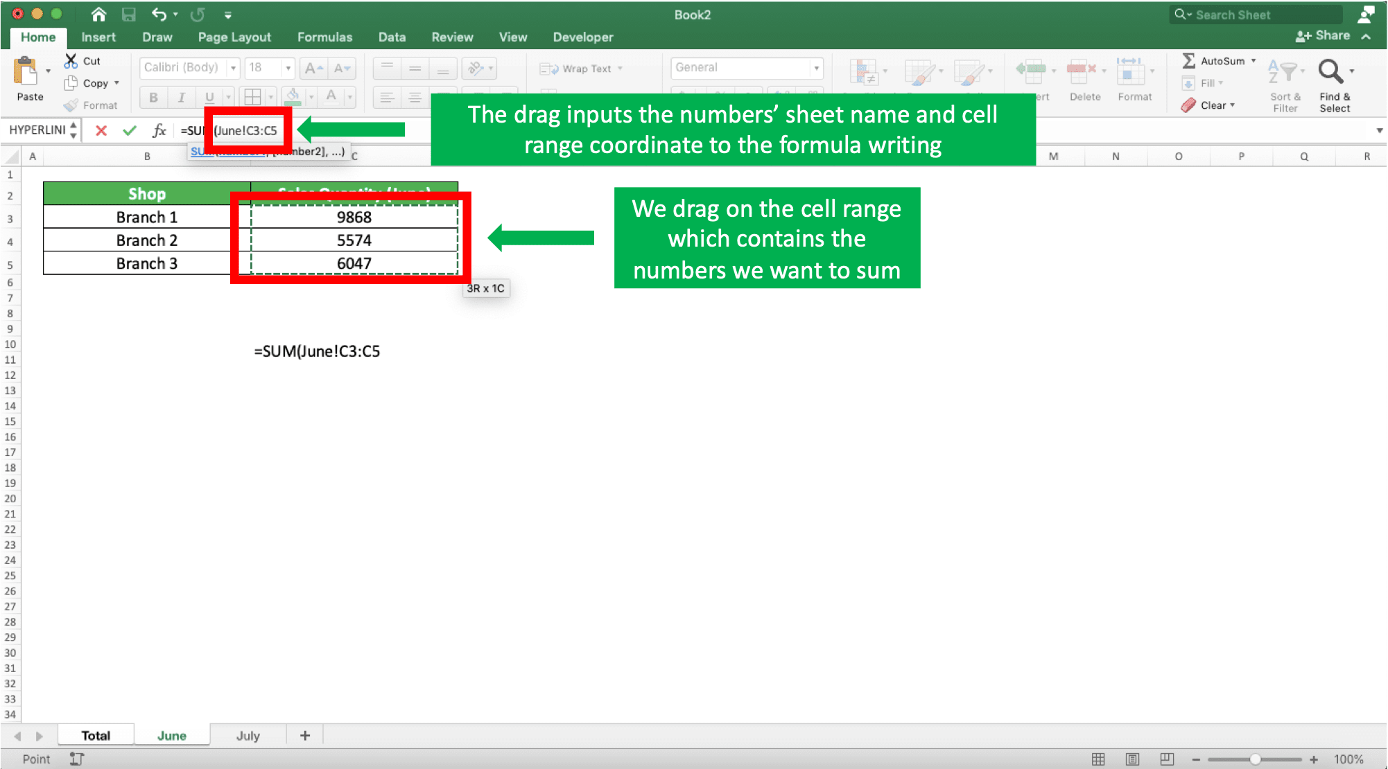
After we input all the numbers we want to sum in SUM, press enter. You will immediately get the sum result!
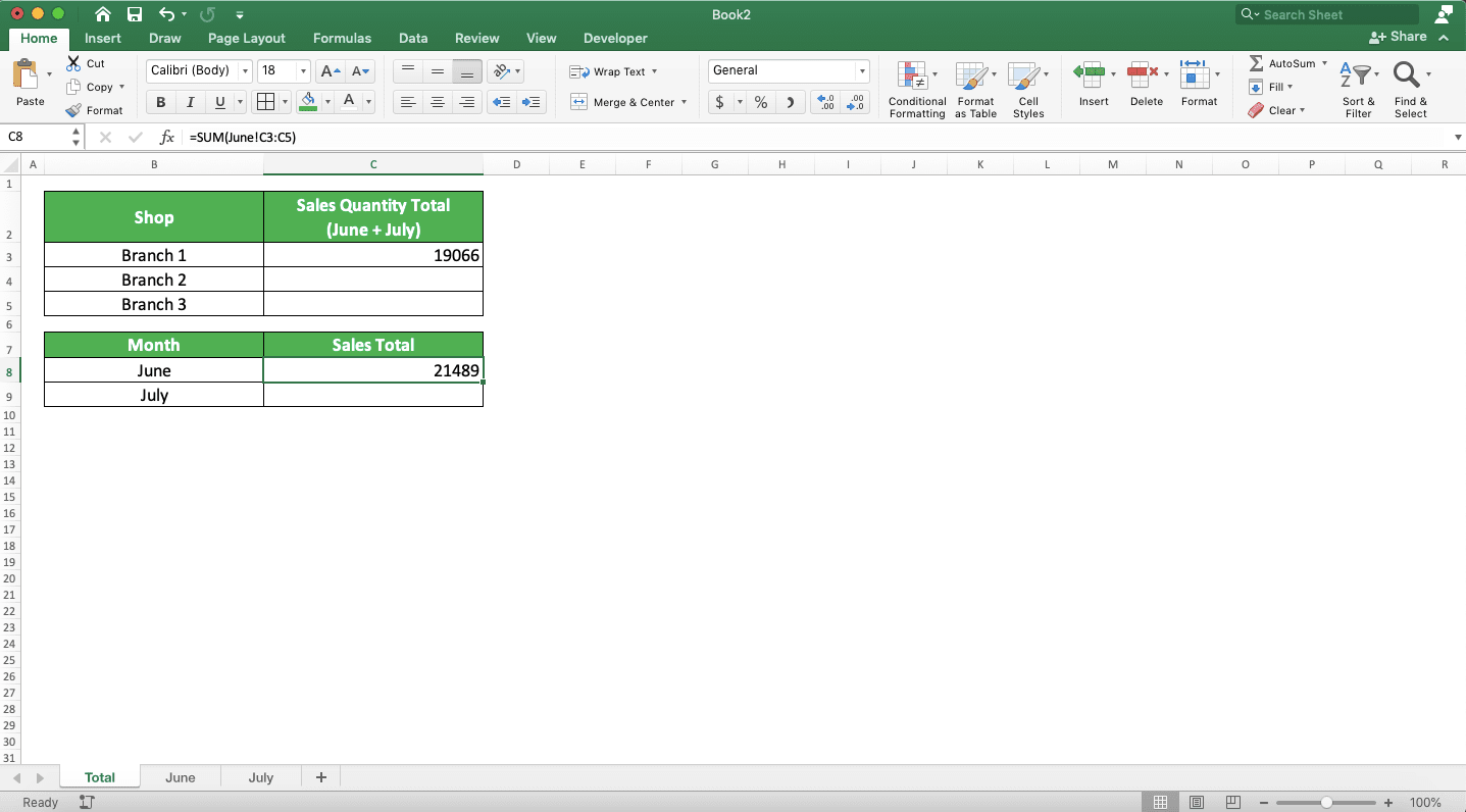
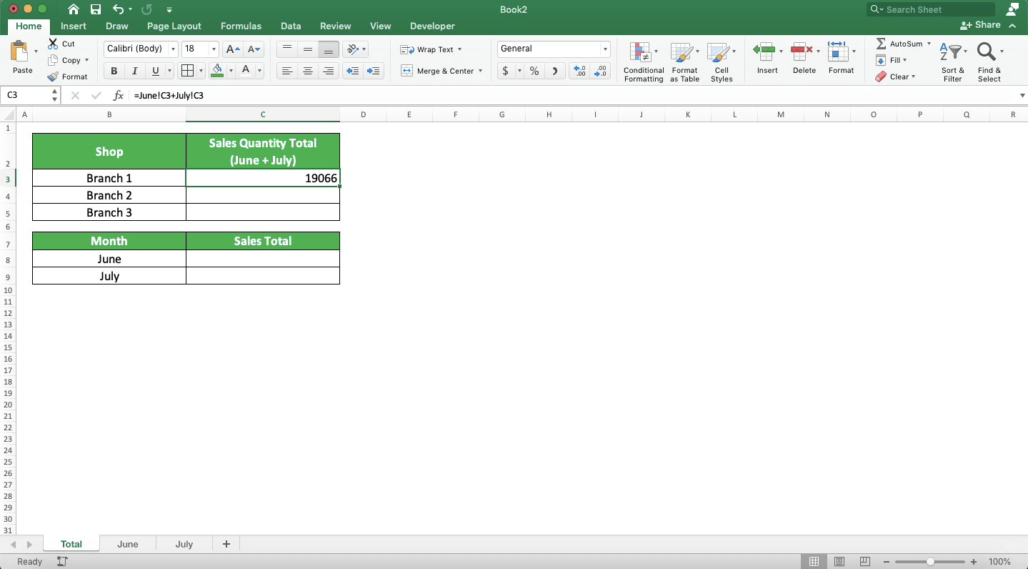
We do all that for all the sum results we need in the “Total” sheet. The result will be like this.
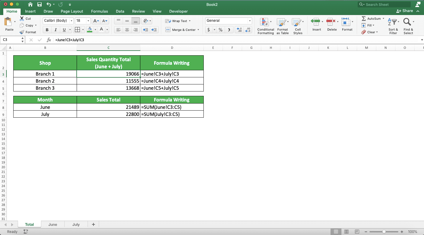
Not too hard, isn’t it?
How to Sum Time in Excel
When processing data in excel, sometimes we have time data and we need to add to them. Maybe we want to add 30 minutes or 2 hours to the time data we have.If you add your time data with a normal number in excel, then you cannot get the result you want. To add to time data, you need to use time data too.
As an illustration of that, look at the following screenshot.
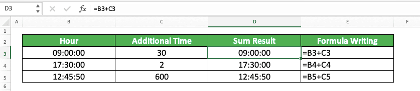
We see there how we want to add to the time data we have.
We want to add 30 minutes, 2 hours, and 600 seconds to each row of our time data. But, because we use normal numbers to add to them, we don’t get the results we want.
Let’s compare to if we use time data to add to the time data we have.
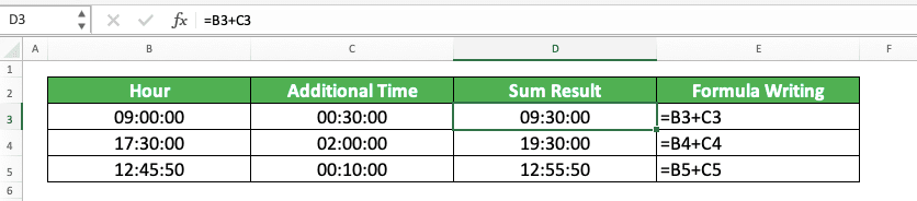
In the second screenshot, we are able to add to the time data. This is because we sum our time data with time data too. The hours, minutes, and seconds we want to add are rewritten in time forms as you can see above.
So, if you want to add to your time data, don’t forget to change all the numbers into time data first!
How to Sum in Excel Using 1 Criterion: SUMIF
Have a criterion for the data entries which numbers you want to sum? You can use SUMIF to help you get the sum result easier.In general, here is the writing form of SUMIF in excel:
=SUMIF(data_range, data_criterion, number_range)
In SUMIF, there are 3 inputs you must give. These are the data column/row cell range you want to evaluate, the criterion, and the numbers column/row cell range.
In the process, SUMIF will evaluate each data in the first cell range you input based on the criterion. If it passes, then SUMIF will sum the number in parallel with the data in the number cell range. With this, SUMIF can sum the numbers which data entries pass the criterion you have.
About the criterion input in SUMIF itself, you must input it correctly so you can get the result you need. You can see the writing examples of a SUMIF criterion and the meaning of them below.
Text (not case-sensitive)
| Criterion Example | Explanation |
|---|---|
| "Jim" | The same as “Jim” |
| “<>Jim” | Not the same as “Jim” |
| “Jim*” | With “Jim” prefix |
| “*jim” | With “jim” suffix |
| “J*m” | “J” prefix and “m” suffix |
| “Jim?” | “Jim” prefix with any one character suffix |
| “?jim” | Any one character prefix with “jim” suffix |
| “J?m” | “J” prefix, any one character, and “m” suffix |
| “Jim~*” | The same as “Jim*” |
| “Jim~?” | The same as “Jim?” |
A bit explanation of the symbols we can use for the text criterion:
- * = represents any character with any amount
- ? = represents any one character
- ~ = use this when you want to add * or ? character for the criterion
Number
| Criterion Example | Explanation |
|---|---|
| 70 | Equal to 70 |
| “>70” | More than 70 |
| “<70” | Less than 70 |
| “>=70” | More than or equal to 70 |
| “<=70” | Less than or equal to 70 |
Date
| Criterion Example | Explanation |
|---|---|
| “>”&DATE(2019,12,3) | Later than 3 December 2019 |
We don’t recommend inputting a date criterion using direct typing (e.g. “>3-12-2019”). t can produce a wrong and unexpected result.
Cell coordinate
| Criterion Example | Explanation |
|---|---|
| “>”&B1 | More than the value in B1 |
Empty/non-empty cell
| Criterion Example | Explanation |
|---|---|
| “" | Empty |
| “<>" | Not empty |
Use the correct criterion writing that fits your sum needs when using a SUMIF!
To make it clearer about this SUMIF, take a look at its implementation example in excel below.
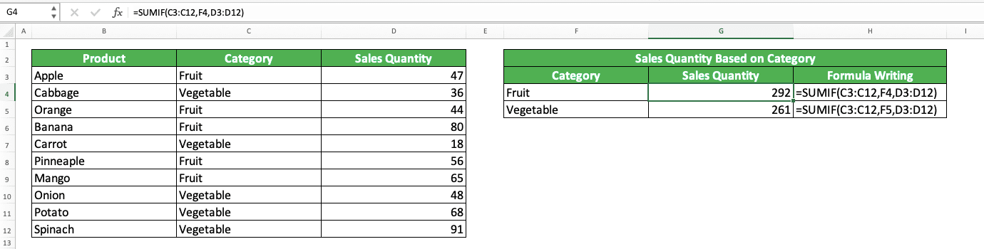
In the example, we want to know the total sales quantity per product category (fruit and vegetable). To get them, we use SUMIF.
As explained before, the SUMIF input begins with the data cell range we want to evaluate based on our criterion. Because, here, the criterion is the product category (vegetable/fruit), we input the cell range where the product category data is. This means the cell range we input is the product category data column.
We input the criterion input based on the product category we want to sum the sales quantity of (fruit or vegetable). And for the number cell range, we input the sales quantity column cell range.
SUMIF will sum all the numbers that are in parallel with the product category we want. Because of that, we get the sum result we want!
How to Sum in Excel Using More than 1 Criterion: SUMIFS
We can use SUMIF if we only have 1 criterion for our sum process. What if we have more than 1 criterion?The answer is you need to use the sibling formula of SUMIF in excel, which is SUMIFS.
Generally, here is the SUMIFS writing form in excel.
=SUMIFS(number_range, data_range_1, criterion_1, …)
In SUMIFS, the data cell ranges we want to evaluate based on our criteria and the criteria are made in pairs. The criterion we input after a cell range will only evaluate the data in that cell range.
Because of that, you need to input the cell range and the criteria according to the number of criteria you need. SUMIFS will sum the numbers in parallel with the data that fulfill all the criteria you have. Just one parallel data that doesn’t pass its criterion and SUMIFS won’t involve the number in its sum process.
The criterion writing of SUMIFS itself is the same as the criterion writing of SUMIF which we have explained earlier.
To better understand the SUMIFS implementation in excel, here is the example.
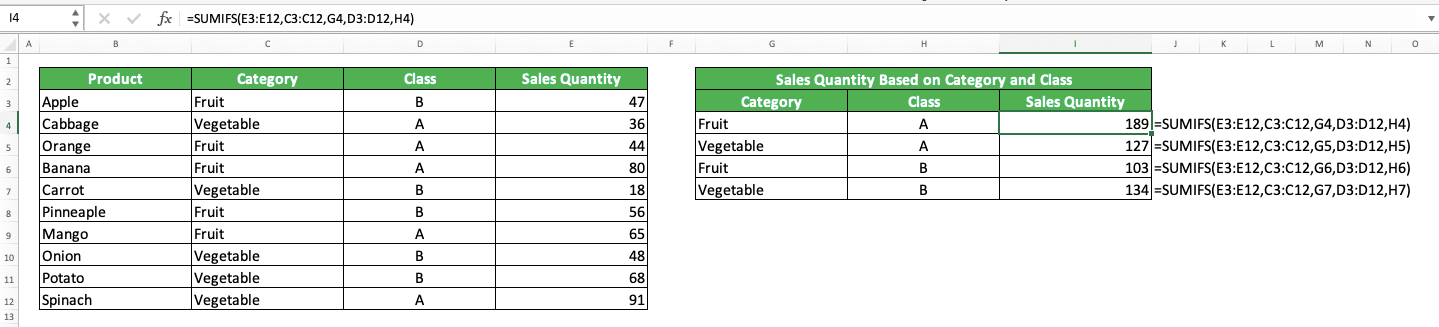
In the example, we have 2 criteria for the sum process, the product category and class. Because of that, we use SUMIFS to help to add the numbers that fulfill both criteria.
We input the sales quantity column we want to sum first, followed by the data columns and their criteria. The data columns and criteria inputs begin with the category column and its category criterion. Then, we input the product class column and its criterion.
Don’t make a mistake when pairing the data cell ranges and the criteria because that will affect your sum result. Don’t forget to input parallel number and data cell ranges that have the same size in SUMIFS. This is so you can predict the result you get much easier.
Give your inputs correctly in the SUMIFS formula you use. You will get the sum result you want as seen in the example above!
How to Sum in Excel for Filtered Data: SUBTOTAL
What if you have filtered the numbers in your data table and you want to sum those filtered numbers?Excel provides a special formula to process filtered data like that, which is SUBTOTAL. We can also use it to sum the filtered numbers that we have!
The general writing form of SUBTOTAL to sum filtered numbers is as we can see in the following.
=SUBTOTAL(9/109, filtered_cell_range_1, …)
The 9/109 input in the SUBTOTAL is a code to make SUBTOTAL sum the numbers of your filtered cell range. Input 9 if you want to sum the numbers from the cells you hide manually too (not hidden by the filter process). If you want to ignore the numbers in those manually hidden cells, input 109.
In SUBTOTAL, the filtered cell range input containing the numbers you want to sum can be more than 1. SUBTOTAL will sum all the numbers from the cell ranges you input in it to give its result.
To make it clearer about the use of SUBTOTAL in summing filtered numbers in excel, look at this example.
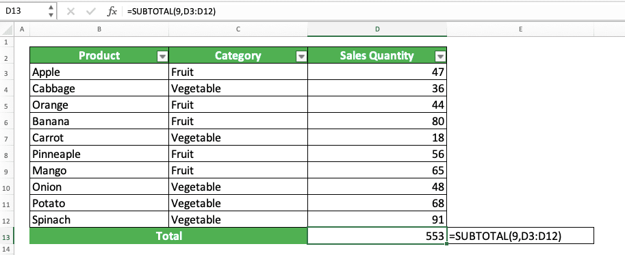
In the example, we want to get the numbers sum result from the sales quantity column with SUBTOTAL. Because we haven’t filtered the table data in the screenshot above, SUBTOTAL will sum the numbers normally.
However, if we filter the data table based on, for example, the fruit category, then the SUBTOTAL result becomes like this.
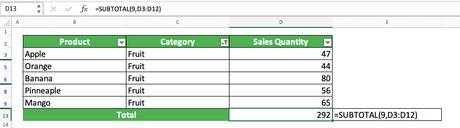
Different compared to the first screenshot’s result, isn’t it? Because we use SUBTOTAL, we will get the sum result of only the numbers that pass the filter. In this example, we will get the sum result of the sales quantity from the fruit category only, which is 292.
The 9 or 109 input in SUBTOTAL in this example will give the same result. This is because there is no row that we hide manually in the data table (all the hidden rows are hidden by the excel filter process).
How to Sum in Excel By Ignoring Errors: SUM IFERROR
Sometimes, in the number sequence we want to sum in excel, there are errors. That sometimes happens if the number sequence is a result of a data processing process.If we want to use SUM to sum the number sequence, then the result will be an error. This is because SUM cannot add an error in the sum process that it does.
We can clean our data first before we sum it, but the process can take time. This is more so if there is much data we must check and clean one-by-one.
Is there any fast way to sum numbers in a cell range that might have errors in it? One of the ways we can implement is by combining our SUM formula with IFERROR.
Generally, here is the writing form of both formulas combined to sum a cell range with errors in it.
{=SUM(IFERROR(number_error, 0))}
We put the cell range containing numbers and errors in IFERROR before we process it with SUM. By using IFERROR like in the writing above, each error will be replaced by 0. Because of that, SUM can process the cell range that contains some errors.
In this formula combination, we use an array formula form (marked with curly braces outside the SUM and IFERROR). We need this form because we use a cell range input in IFERROR which usually processes individual data.
To change our formula writing form into an array, we press Ctrl + Shift + Enter after we write the formula (not pressing enter like when we write a normal formula).
To better understand this SUM IFERROR implementation, see the following example.
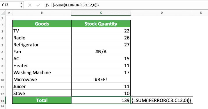
In the example’s stock quantity column, there are two errors among the numbers we want to sum. If we use a normal SUM to get the total stock quantity, we will get an error result.
Because of that, we use IFERROR in the SUM formula writing. By changing each error in the cell range we want to sum with 0, we can get our sum result
How to Sum Much Faster in Excel: AutoSum
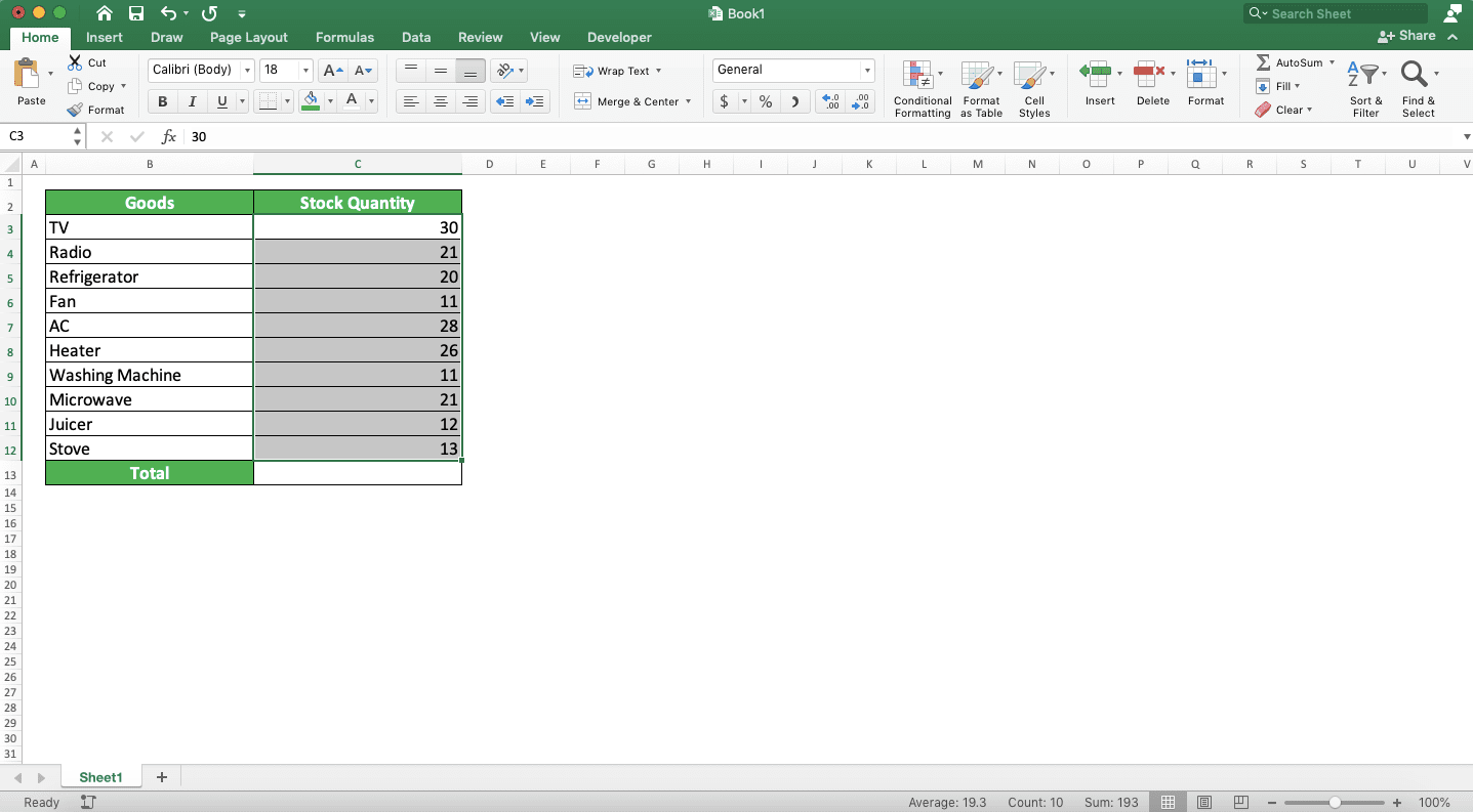
If you want to sum a number sequence in an excel column/row, there is a fast way to do it. The fast way is by utilizing the AutoSum feature from excel. By using AutoSum, you will immediately get a SUM writing containing the number sequence’s cell range input.To make it clearer about this AutoSum usage in excel, take a look at the following steps.
First, highlight your number sequence or place your cell cursor one cell outside the number sequence you want to sum.
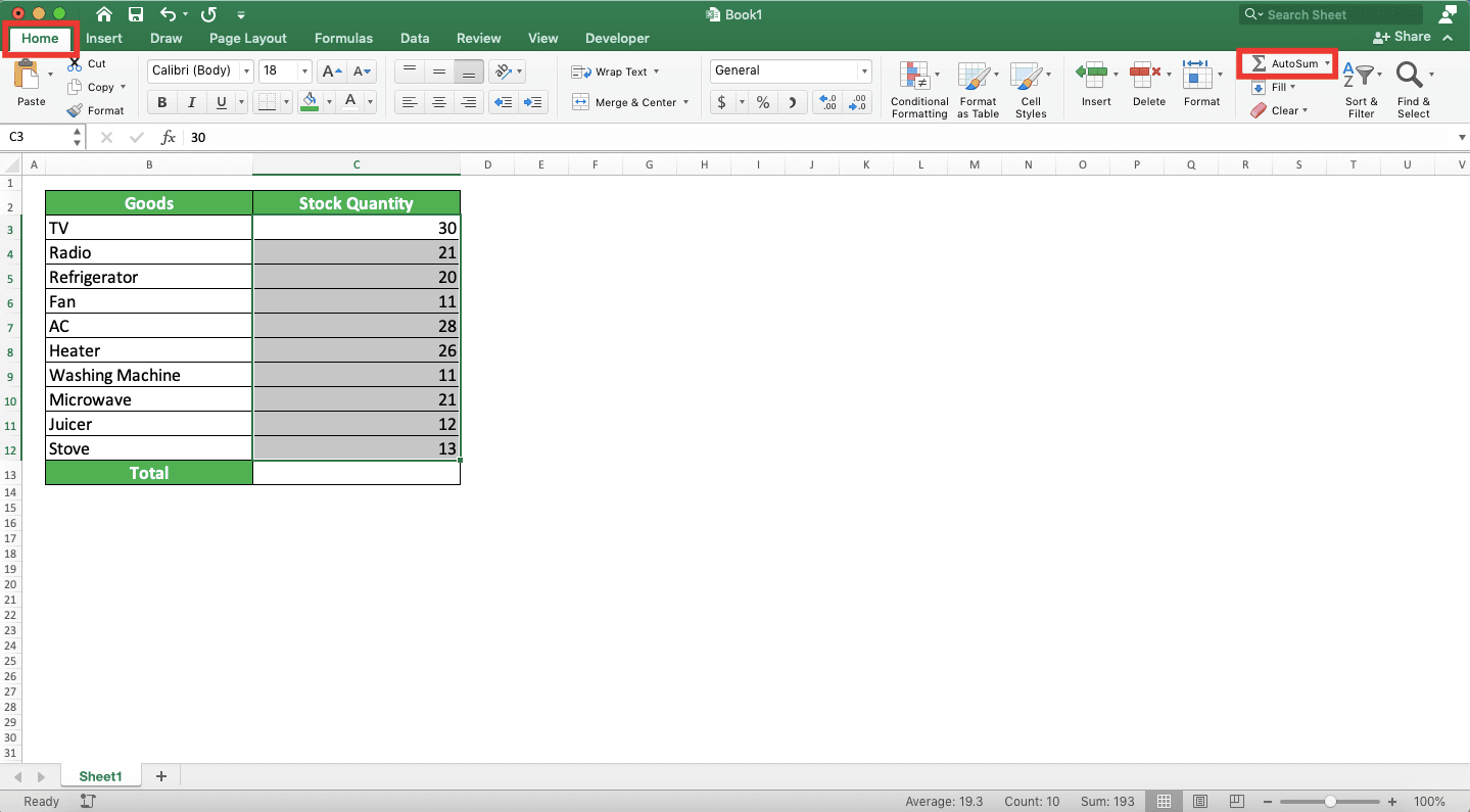
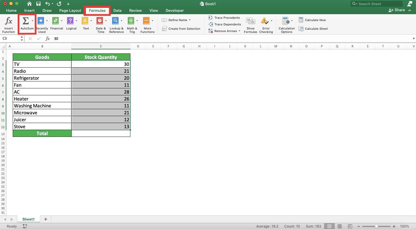
Next, activate the AutoSum feature. How? You can activate it by going to the Home or Formulas tab and click on the AutoSum button there. You can also use a shortcut by pressing the Alt and = (Windows) / Command, Shift, and T (Mac) buttons simultaneously.
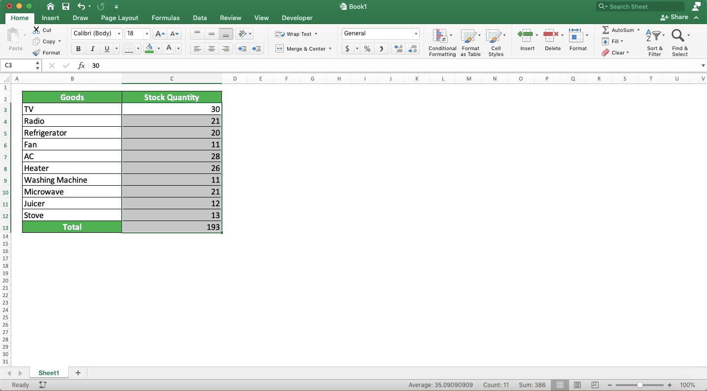
Excel will automatically produce a SUM formula that sums your number sequence. The SUM writing will be placed one cell outside your number sequence!
Exercise
After you learn how to sum in excel completely from the tutorial above, sharpen its implementation understanding by doing this exercise!Download the exercise file from the link below and answer the questions. Download the answer file to check your results if you have done the exercise and sure about your answers!
Link of the exercise file:
Download here
Questions
- How many is the number of total students from all classes?
- How many is the number of total students for class A? Use SUMIF to answer!
- How many is the number of total students for class 2 and 3 with code B? Use SUMIFS to answer!
Link of the answer key file:
Download here
Additional Note
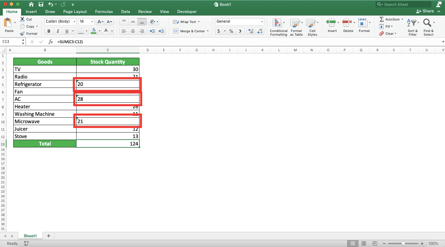
Make sure the numbers you want to sum aren’t in text forms!This text number problem sometimes shows up, especially if the numbers are from external sources. The text forms of your numbers will make them not summed when you want to sum them with other numbers!
Excel usually marks a text number with a green triangle on the top left of its cell like this.
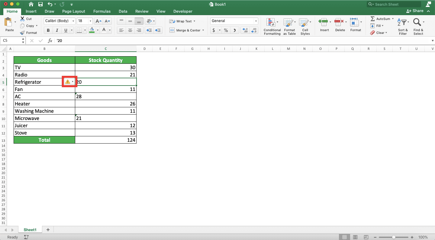
What if you want to change a text number into a normal number? You can begin to change it by placing your cell cursor in the cell containing the text number. Usually, there will be a box with an exclamation mark triangle that shows up like this.
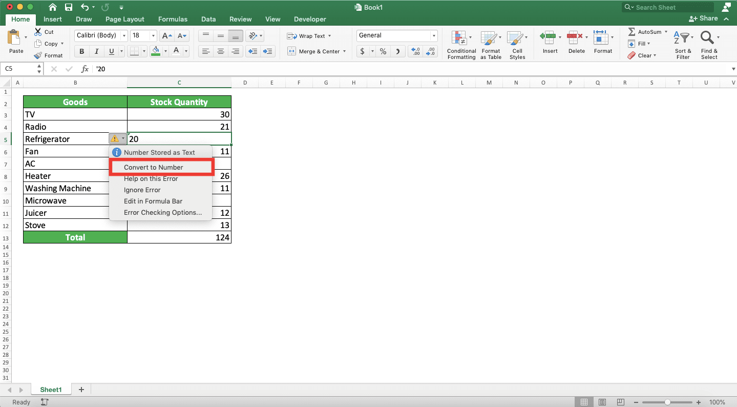
You just need to click on the box and choose Convert to Number from the choices that show up.
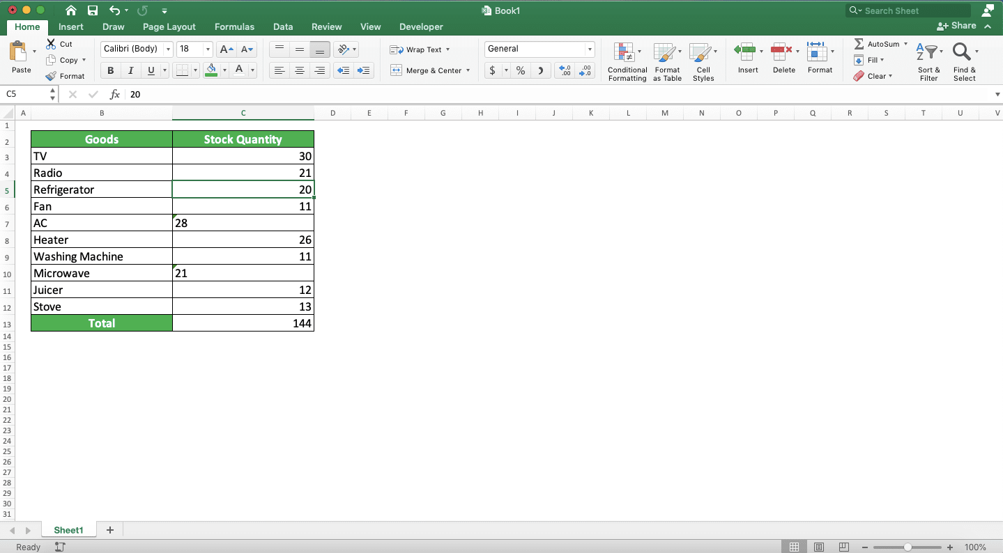
The text number in the cell will be converted to a normal number!
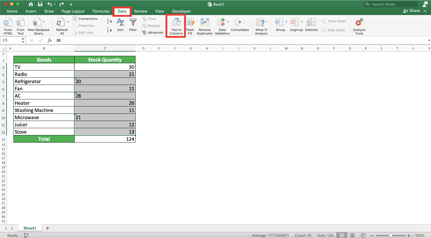
If there are many text numbers in the cell range you want to sum, use this method to convert them simultaneously. Highlight the cell range, go to the Data tab, and choose Text to Columns.
Then, click Finish in the dialog box that shows up.
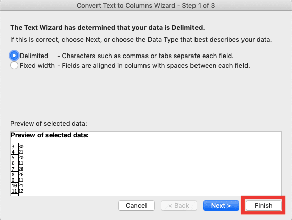
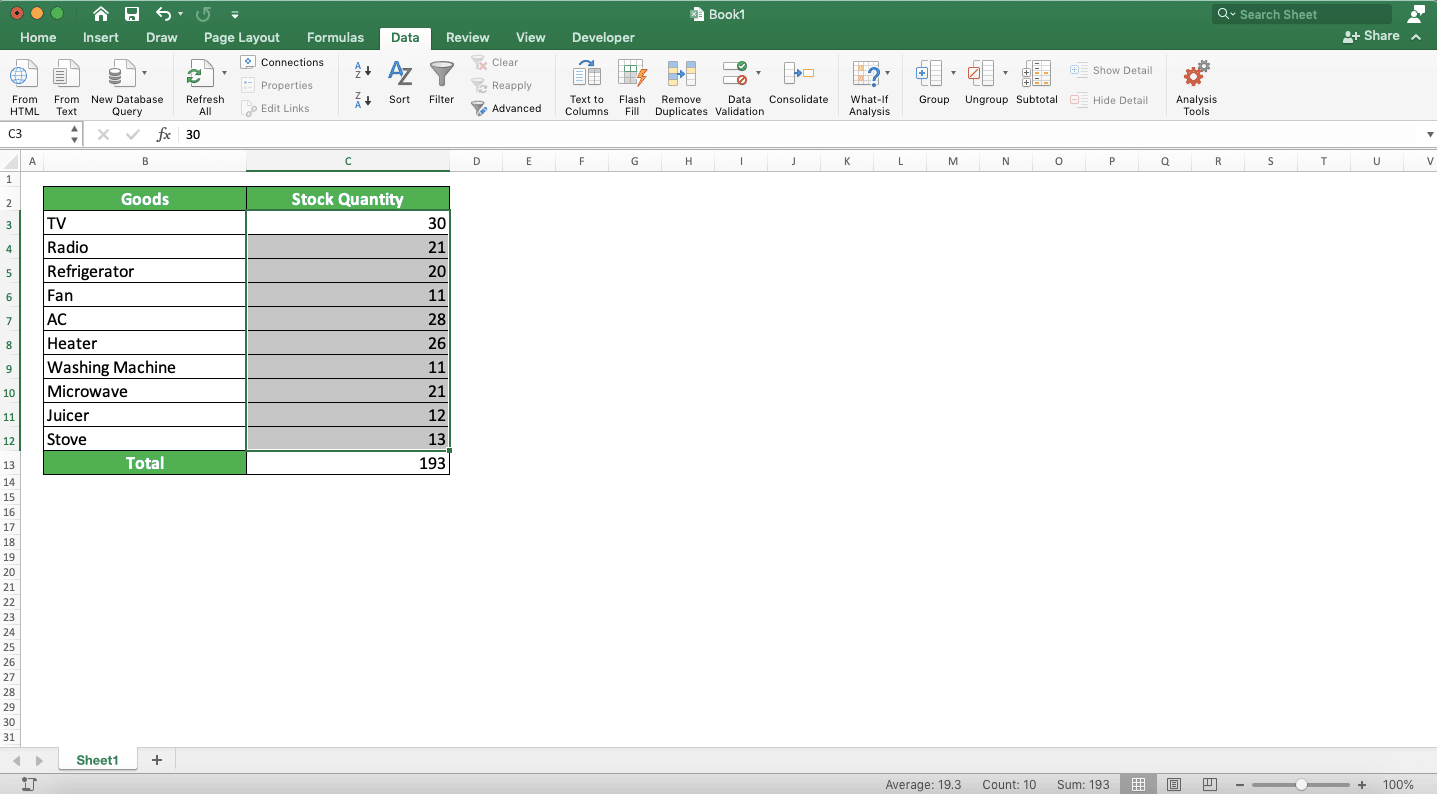
Excel will immediately convert the text numbers in the cell range you highlight to normal numbers!
Related tutorials you should learn