How to Use SUMIFS Excel Formula: Function, Examples, and Writing Steps

In this tutorial, you will learn completely about the SUMIFS excel formula. We will discuss its function, examples, writing steps, and use cases here.

If you have some criteria for the data entries which numbers you want to sum, then this is your formula. SUMIFS can do that kind of sum process for you in a blink, assuming you have mastered the formula usage.

Want to understand how to use the formula so you can use it optimally? Follow this tutorial until its last part!

Disclaimer: This post may contain affiliate links from which we earn commission from qualifying purchases/actions at no additional cost for you. Learn more

Want to work faster and easier in Excel? Install and use Excel add-ins! Read this article to know the best Excel add-ins to use according to us!

SUMIFS Definition

We can define SUMIFS as a formula that can help us to sum numbers from selected data entries. The selection of the data entries depends on the criteria we give as inputs to SUMIFS.

SUMIFS Excel Function

SUMIFS function in excel is to sum numbers from data entries that meet our criteria.

SUMIFS Result

SUMIFS result is a number that represents the sum of numbers from data entries that meet our criteria.

Excel Version from Which We Can Use SUMIFS

We can start to use SUMIFS since excel 2007.

The Way to Write It and Its Inputs

We can write SUMIFS in an excel cell with the form like this one.



And here is the explanation of the inputs which we should give in the SUMIFS writing.

• sum_range = the cell range where the numbers of the selected data entries that we want to sum are
• data_range1 = the cell range which data will be evaluated by your first criterion
• criterion1 = the first criterion
• … = other cell range and criterion pairs

We usually input the cell ranges in SUMIFS in the form of parallel rows or columns. The cell ranges inputs must be in the same size (have the same numbers of rows and columns) and should be parallel.

Example of Its Usage and Result

Here is an example of the SUMIFS implementation in excel with its result.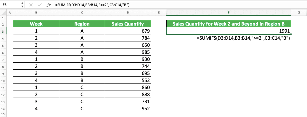



In this example, we want to sum the sales quantities for region B on weeks 2-4. For this, SUMIFS can help us significantly to get the result we want.

We just need to input the correct number range and also the correct data range and criterion pairs into the SUMIFS. In this case, the numbers we want to sum are the sales quantities. Therefore, we input the sales quantities column as the number range.

We have the criteria of region B and weeks 2-4 for this sum process. Thus, we input the region column and the week column for the data ranges. For the criteria that follow them, we input “B” for the region and “>=2” for the week (which signifies more than 2 as a criterion in excel).

The SUMIFS writing result with those inputs is as you can see in the example. Write the formula correctly and you will get the sum result you want from your SUMIFS!

Criteria Writing in SUMIFS

There can be many kinds of criteria we want to input to SUMIFS depending on our sum condition. Those criteria can require different kinds of writing too. You must get the correct writing for your criteria so you can get the correct result too from your SUMIFS.



How can I write the criteria that I want in SUMIFS? Well, we have gathered the list of excel criteria writing examples and their meanings. Find the writing which suits your SUMIFS needs through this list!

Text (not case-sensitive)

Criterion Example	Explanation
"Jim"	The same as “Jim”
“<>Jim”	Not the same as “Jim”
“Jim*”	With “Jim” prefix
“*jim”	With “jim” suffix
“J*m”	“J” prefix and “m” suffix
“Jim?”	“Jim” prefix with any one character suffix
“?jim”	Any one character prefix with “jim” suffix
“J?m”	“J” prefix, any one character, and “m” suffix
“Jim~*”	The same as “Jim*”
“Jim~?”	The same as “Jim?”

A bit explanation of the symbols used in some of the text criteria:

• * = any character with any amount
• ? = any one character
• ~ = used when you want to add a literal * or ? character in the criterion

Number

Criterion Example	Explanation
70	Equal to 70
“>70”	More than 70
“<70”	Less than 70
“>=70”	More than or equal to 70
“<=70”	Less than or equal to 70

Date

Criterion Example	Explanation
“>”&DATE(2019,12,3)	Later than 3 December 2019

It isn’t recommended to input a date criterion with direct writing (e.g. “>3-12-2019”). The reason is that direct writing can produce a wrong and unexpected result.

Cell coordinate

Criterion Example	Explanation
“>”&B1	More than the value in B1

Empty/non-empty cell

Criterion Example	Explanation
“"	Empty
“<>"	Not empty

Writing Steps

After discussing the SUMIFS implementation example and its criteria writing, now let’s discuss its writing steps. After reading this part, you should understand how to write perfect SUMIFS in excel.

We discuss each step here with its screenshot example to make you understand the steps easier!

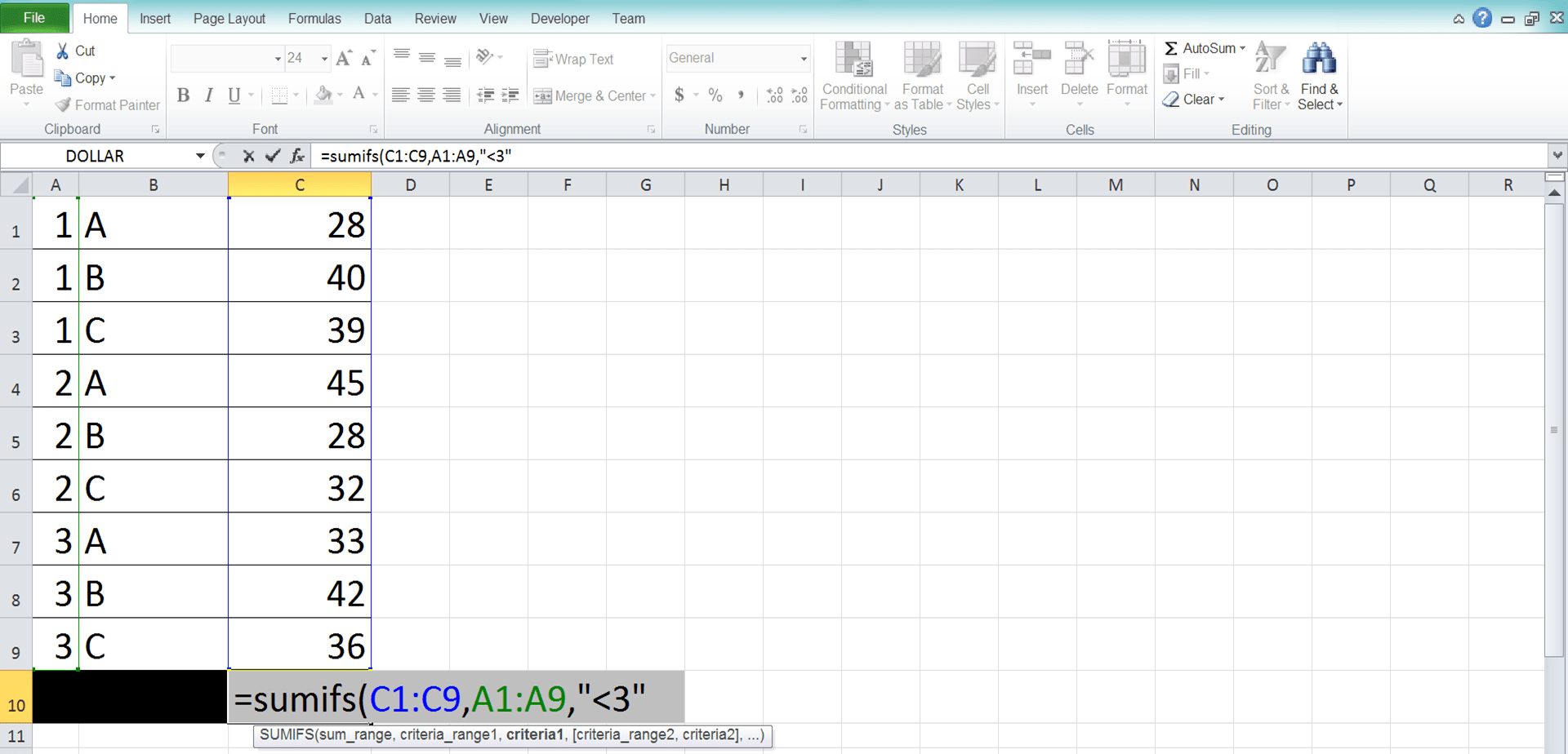
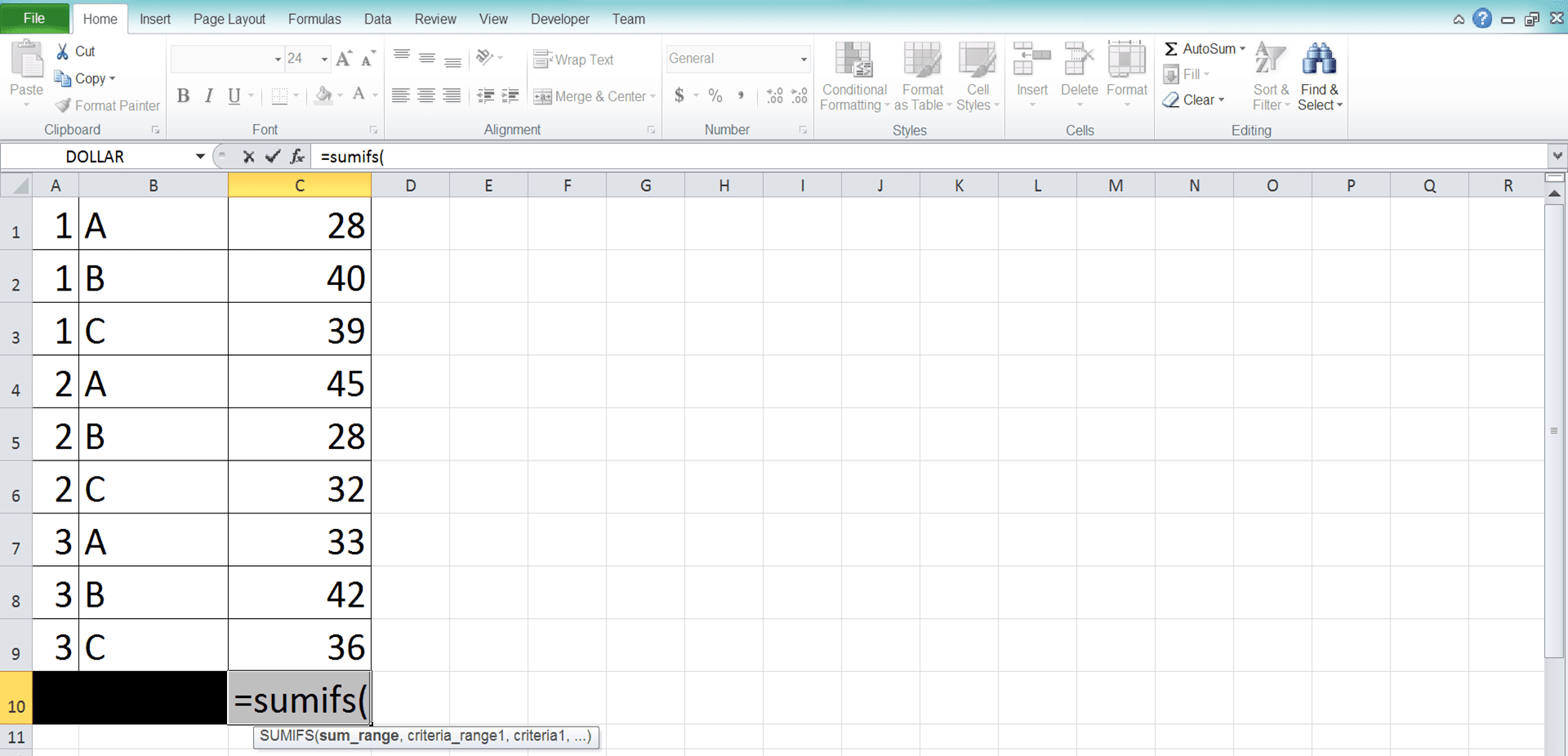
1. Type an equal sign ( = ) in the cell where you want to put the SUMIFS result
   
   
   
   
2. Type SUMIFS (can be with large and small letters) and an open bracket sign after =
   
   
   
   
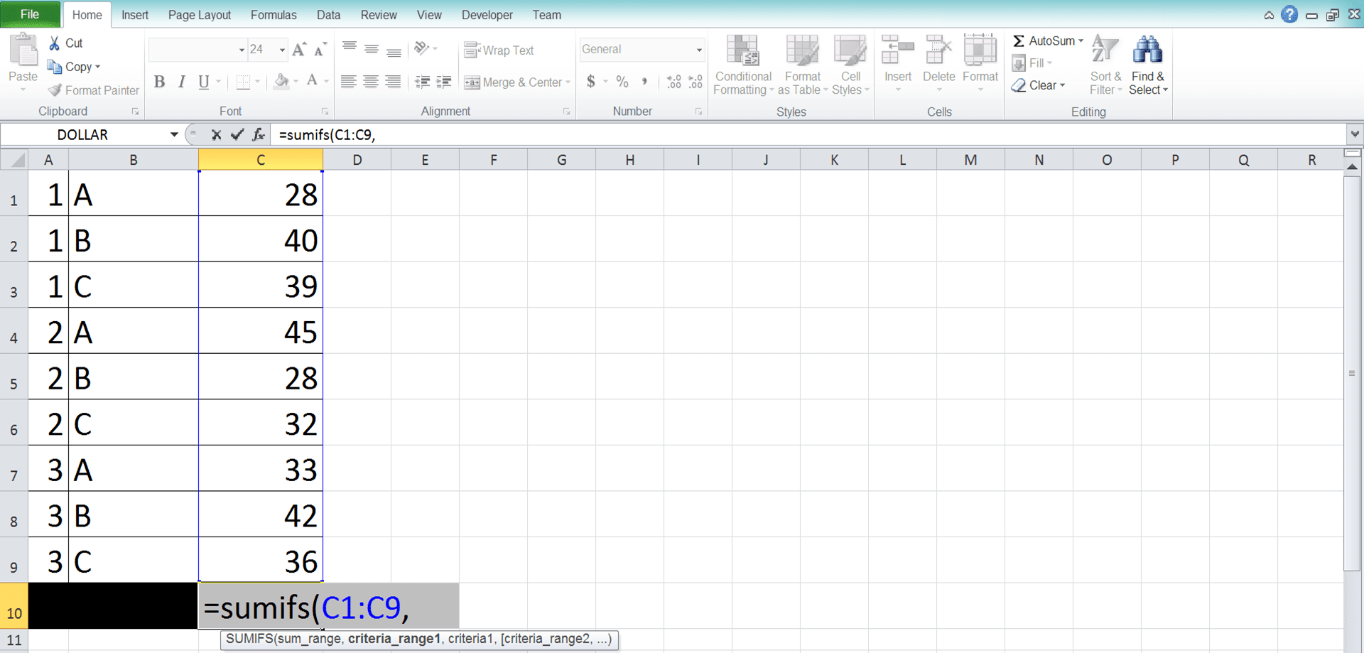
3. Input your number range, the cell range where the numbers you want to sum from your data entries are. Then, type a comma sign ( , )
   
   
   
   
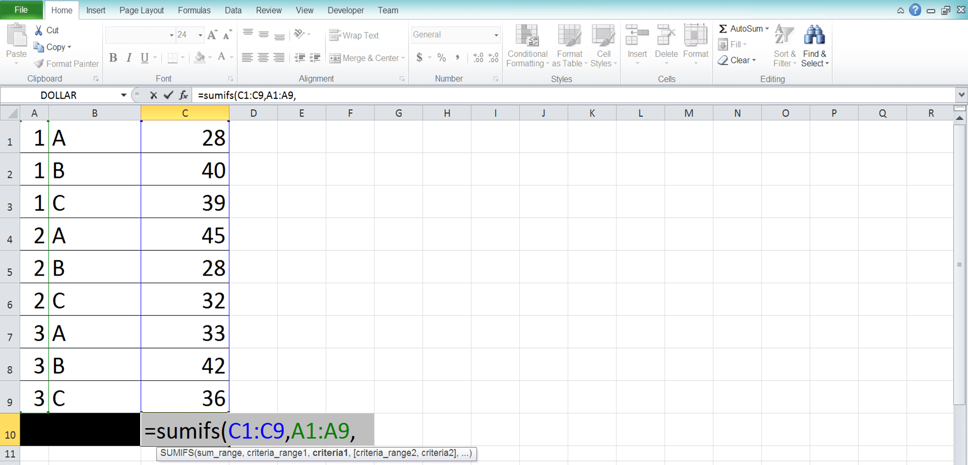
4. Input your first data range, the cell range which data you want to evaluate with your first criterion. It should have the same size and be parallel with the number range you inputted earlier. Then, type a comma sign
   
   
   
   
5. Input your first criterion, the one you use to evaluate the data in the cell range you inputted just now
   
   
   
   
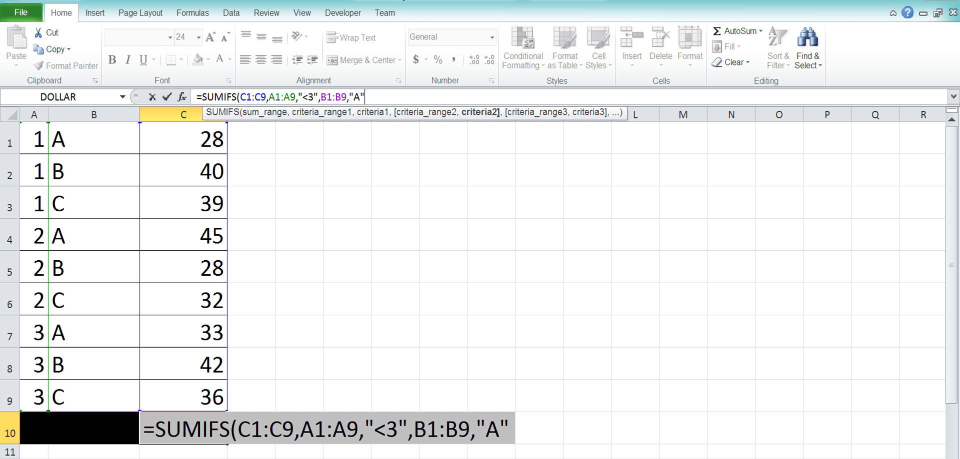
6. Optional: if you still have other criteria, then do this. Type a comma sign and redo steps 4-5. Do this until you have inputted all of the data range and criterion pairs you need
   
   
   
   
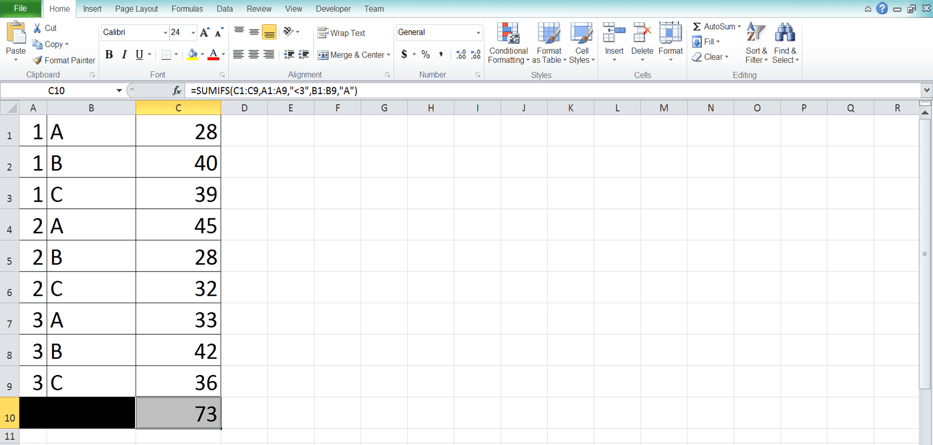
7. Type a close bracket sign after you have inputted all your data range and criterion pairs
   
   
   
   
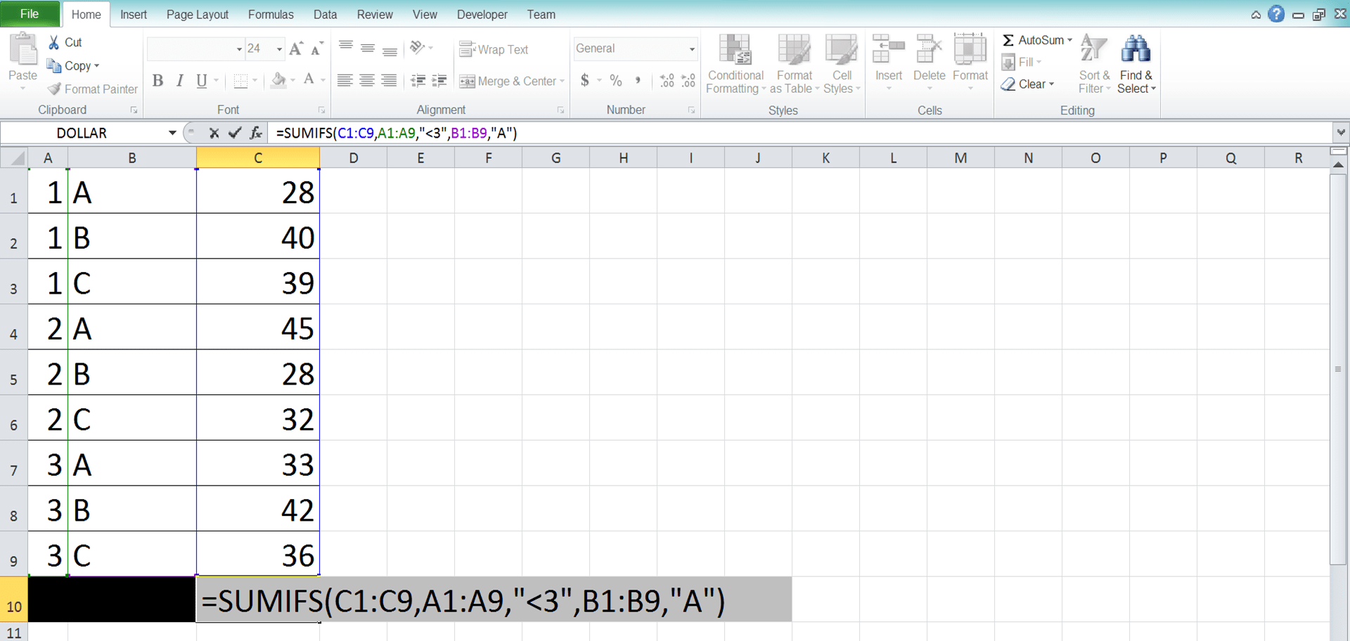
8. Press Enter
9. Done!
   
   
   
   

The Reasons Why Your SUMIFS Doesn’t Work Properly

Get a wrong or error result from your SUMIFS? Then, you most probably have written your SUMIFS incorrectly!

There are many factors that can make your SUMIFS writing produces a wrong or error result. However, these three below seem to be the most frequent reasons.

• You have inputted the wrong cell range and criterion pairs. Remember, that the criteria you input only evaluate the data from the cell range input before it. Check your data ranges and criteria input order and make sure you don’t input the wrong cell range and criterion pairs!
• You have written your criteria wrongly. Check them by referring to the criteria writing examples we discuss previously. Make sure SUMIFS can use your criteria writings just the way you want it to
• You didn’t input parallel and same size cell ranges in SUMIFS. This can often cause SUMIFS to produce an error/wrong result

Check again your SUMIFS and make sure you don’t do the mistakes above!

SUMIFS with Multiple Criteria in the Same Column

SUMIFS allows you to evaluate different columns with a different criterion for each to sum the numbers you want. However, what if we have more than one criterion for a column? How should we do the inputs on this kind of condition into our SUMIFS?

If those criteria for a column have an AND nature (our data in the column must fulfill all the criteria to pass), then input the criterion with the same data range. However, if those criteria have an OR nature (our data in the column can fulfill only one of those criteria to pass), then you must create multiple SUMIFS to be summed later.

To make you understand the concept easier, here is an example for both of AND and OR nature.



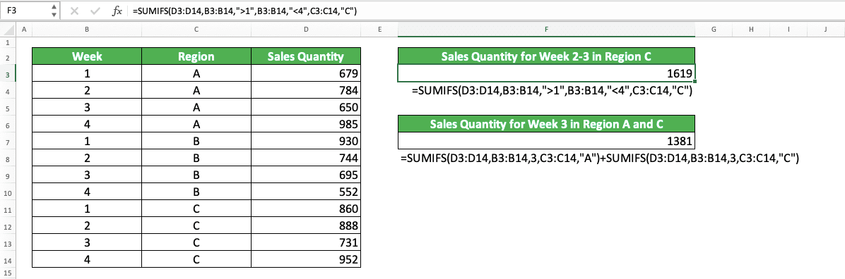
As you can see in the screenshot, we have two conditions for our sum process. The first is to sum sales quantities from week 2-3 in region C. The second one is to sum sales quantities from week 3 in region A & C.

For the first condition, we cannot input just one criterion into SUMIFS as we cannot write a range criterion directly. The way to write the range is by breaking it down into two criteria, “more than” and “less than”.

Thus, this is what we do. We break the week 2-3 range into more than 1 (“>1”) and less than 4 (“<4”).

As the criterion is a range, our week data must fulfill all those broken down criteria to pass. This is an example of the AND nature for multiple criteria for one column in SUMIFS. Because of that nature, we input the week cell range twice with the “more than” and “less than” criteria for each.

For the second condition, we use multiple SUMIFS to handle the sum process. This is because the nature of the multiple criteria in the same column here is OR. The multiple criteria are for the region data and it can be B or C for this sum process.

Therefore, we write SUMIFS for each of the region criteria. One for the “B” region criterion and one for the “C” region criterion.

Other inputs in the two SUMIFS are the same besides those region criterion.

Write the formula correctly like that and we will get the sum result that we want!

SUMIFS Across Multiple Sheets

In excel, we may have our data divided into sheets. For example, we may divide our company spending data into months and those months are translated into different sheets in excel. That division can make it much easier for us to navigate our excel file and find the data we need.

However, we may find a problem when we need to apply SUMIFS to the numbers in those different sheets. We don’t know how to pull those numbers from their sheets to get the sum result we need.

For this, you need to use the SUMIFS method to sum across multiple sheets.

We will use the help of INDIRECT and SUMPRODUCT formulas to help us with this kind of sum process using SUMIFS. Here is the general writing form for the combination of those three formulas for the purpose.



For this formula writing, we should list the sheet names where we want to pull our numbers in a cell range. That will make it easier for us to sum them instead of having to write the sheet names one by one.

We put the sheet names cell range into INDIRECT, together with the cell range of the numbers in those sheets. INDIRECT will change its input into a reference which we can use for our SUMIFS and SUMPRODUCT.

One important thing to note also is the number cell ranges must be the same across the sheets. This is usually a common thing as we often have the same template for the data of those kinds of sheets.

Then, in the writing, we use SUMIFS to get the numbers from those sheets using our criteria. For the data range inputs, we also use INDIRECT to pull the data we want to evaluate with our criteria. The INDIRECT writing pattern for the data ranges is similar to the INDIRECT writing pattern for the number range.



Finally, the SUMPRODUCT there helps INDIRECT to process a cell range input as it usually just accepts individual data input.

Don’t forget to input your criteria correctly in the SUMIFS so you can get the sum result you need!

To help you understand the concept of this SUMIFS application, here is the implementation example in excel.

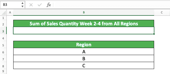
Let’s say we have a sheet where we want to put our multiple sheets SUMIFS result like this.



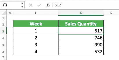
For the data in each of the SUMIFS sheet sources, the template is like this.



How do we get the sum result with the criteria that we have in the result sheet? Well, here is the formula writing using SUMPRODUCT, INDIRECT, and SUMIFS to do that.



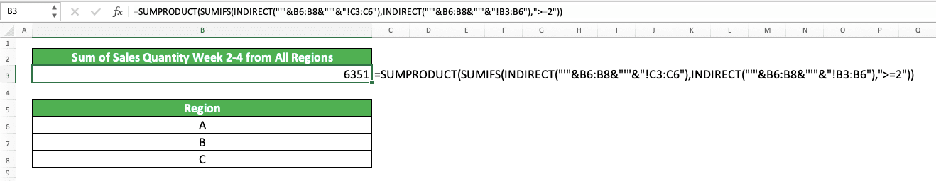
We use INDIRECT to pull the number and data range inputs for SUMIFS in the example. We can do this easier because we have the region column there which specifies all the region sheet names.

We input the region column cell range and input the number and data cell ranges in the region sheets. We also input the week criterion there (“>=2”) to get the sum result we want from SUMIFS.

Last but not least, we write the SUMPRODUCT formula to envelopes the SUMIFS and INDIRECT formulas.

Write them all correctly in your case and you can do this SUMIFS across multiple sheets too!

SUMIFS Between Dates

Date data can sometimes become the criteria we need in our sum calculation in excel. Maybe we want to sum profit from January to March or we want to sum sold products for 2 years.

We can do the sum process using SUMIFS. However, for that, we need to understand how to SUMIFS between dates using the right criteria writing.

In general, the way to write SUMIFS with date range criteria is similar to write SUMIFS with number range criteria. Here is its general writing for illustration.



As with a number range criterion, we split the range to “more than” and “less than” criteria. If you need it, you can also give an “equal to” criterion by adding “=“ behind the “>” or “<“.

We use the DATE formula to help us input the date criterion. This is to make it easier as directly typing the date can cause an error/wrong result.

If you have other criteria than the date range, then you can input it after or before the date criteria.

For the implementation example of the formula writing, you can see it below.



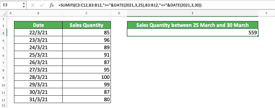
In the example, we want to sum the sales quantities between 25 March 2021 and 30 March 2021. To get the result, we use SUMIFS.

You can see how we write the date range criterion in the formula. We use the “more than equal to” and “less than equal to” criteria to split up the date range criterion.

For the “more than equal to” criterion, we write “>=“&DATE( 2021, 3, 25). For the “less than equal to” criterion, we write “<=“&DATE( 2021, 3, 30). We input the same date range for both of the criteria as they should evaluate the same dates.

From this formula writing, you can see that we get the sum result we want in the example (559 for the sales quantity between 25 March 2021 and 30 March 2021)!

SUMIFS VLOOKUP/SUMIFS INDEX MATCH: Multiple Criteria Lookup

When we discuss a lookup formula in excel, we usually think about VLOOKUP or INDEX MATCH. However, these formulas can only have one criterion as its lookup value reference. It normally cannot help us if we have multiple lookup value references that we need to look to.

In this condition, SUMIFS can help us to do the lookup as it can have multiple criteria inputs. This is true especially if the data you want to find is a number as SUMIFS produces that type of data. However, if you want to find non-number data, then you can just combine SUMIFS with VLOOKUP/INDEX MATCH.



Moreover, your data entries should be unique to each other as complete duplicates can cause SUMIFS to sum instead of find. As we want to look up data, we should avoid the sum process from SUMIFS.

The way to write SUMIFS for the lookup purpose is similar to the normal SUMIFS. We just change the data ranges and criteria inputs to the lookup ranges and lookup values.



We use the cell range where SUMIFS usually gets its numbers into the place where it finds data. For the lookup references, we make it as criteria inputs in SUMIFS. We also specify the cell ranges where SUMIFS should find the lookup references.

As previously explained, this assumes the data you want to find is a number. If it isn’t a number, however, then you can use SUMIFS as a media for VLOOKUP/INDEX MATCH to find it. As long as there is a number range in the data table, then you can utilize SUMIFS to lookup the data.

If you use VLOOKUP with SUMIFS, then ensure the number range is in the first column of its cell range input. This is because VLOOKUP can only look for its lookup reference in the most left column of its cell range input.

We can illustrate the way to write the SUMIFS with VLOOKUP like this.



We write SUMIFS as the lookup reference input for VLOOKUP. As SUMIFS gets its result, it will then give VLOOKUP the input it needs to get the data you want.

We input multiple criteria we have for the lookup in our SUMIFS.

This is also true if we use INDEX MATCH with SUMIFS instead of VLOOKUP.



The writing assumes we have to find the data vertically as we put the MATCH in the INDEX row input. However, you can write the MATCH in the column input part of INDEX too if you need it. We put SUMIFS in the lookup reference of MATCH as it needs to look for multiple criteria for its lookup process.

INDEX MATCH is more flexible than VLOOKUP because you don’t have to get the number range as your first column. Thus, if you understand INDEX MATCH, then you should use it for the data lookup combination with SUMIFS!

To understand clearer about this multiple criteria lookup using SUMIFS, here is the implementation example of the methods in excel.



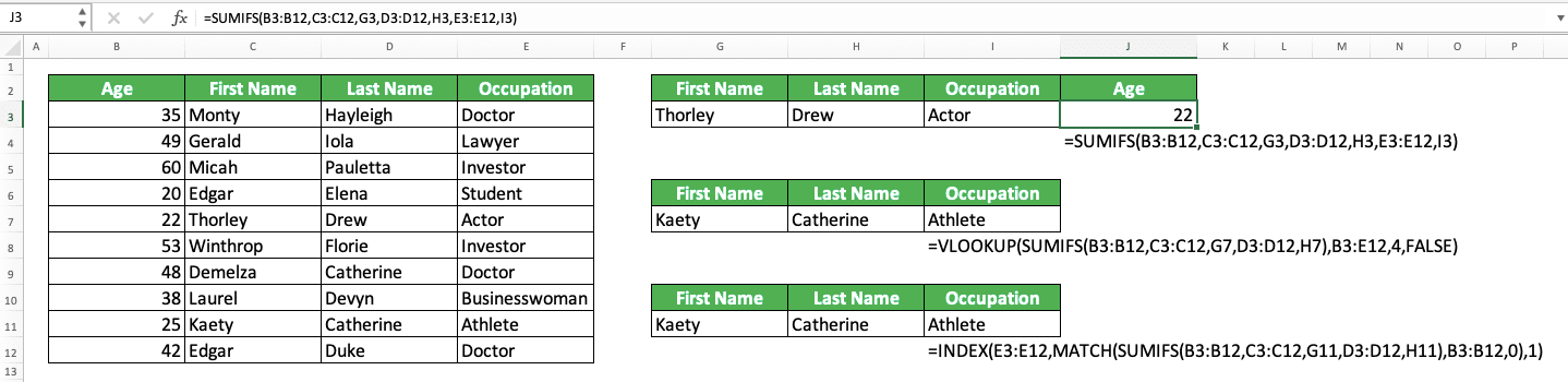
In the example, you can see the practice of the three excel lookup methods using SUMIFS that we have discussed previously. They are the ones using SUMIFS only, SUMIFS with VLOOKUP, and SUMIFS with INDEX MATCH.

We have a data table of people’s age, first name, last name, and occupation here. Using SUMIFS only, we can find the age data of a given person. Just input the age column range, the data cell ranges that we use as criteria, and the criteria themselves. As you can see in the screenshot, we can find the age of Thorley Drew using this method!

What about the one with VLOOKUP/INDEX MATCH? We use it if we want to find non-number data using multiple criteria.

As we see in the example, we also need to look for occupation data using first and last name references. For that, we can use SUMIFS VLOOKUP or SUMIFS INDEX MATCH. We can use SUMIFS VLOOKUP because the age column there is the first column of the data table.

We type our SUMIFS inside the place where we usually input our lookup reference value in VLOOKUP/INDEX MATCH. We also use the number range of SUMIFS as the place where we look for the lookup reference.

This makes us able to locate the row of the data that we want to find at the data table column. As a result, we get the occupation data from both SUMIFS VLOOKUP and SUMIFS INDEX MATCH!

After you understand this concept, you should be able to do multiple criteria lookup in excel much easier!

SUMIF and SUMIFS Difference

Before you visit this tutorial to learn SUMIFS, you may have known about its sibling formula, SUMIF. You can also use SUMIF to sum numbers from data entries that meet your criterion.

Then, what is the difference between the two? Well, the difference lies in the number of criteria we can use. We can only use one criterion for our sum process if we use SUMIF. Meanwhile, we can use one or more criteria if we use SUMIFS.

Can we use SUMIFS instead of SUMIF if we only use one criterion in our sum process? Yes, sure! However, if you use excel 2003, then you can only use SUMIF as SUMIFS is only available since excel 2007.

Exercise

After you learned completely how to use the Excel SUMIFS formula, practice your understanding of using SUMIFS through this exercise!

Download the exercise file from the following link and answer the questions below. Download the answer key file if you have done the exercise and want to check your answers!

Link to the exercise file:
Download here

Questions

1. What is the numbers’ total if we have the criteria of A in the second and fourth columns?
2. What is the numbers’ total for A in the first, B in the third, and C in the fifth column?
3. What is the numbers’ total if the criteria are A, B, C, C, B for first until the fifth column?

Link to the answer key file:
Download here

Additional Note

You can input cell range and criterion pairs in SUMIFS up to 127 pairs.



Related tutorials you should learn: