How to Use COUNTIF Formula/Function in Excel

In this tutorial, you will learn completely about how to use the COUNTIF formula in excel. COUNTIF can help you to calculate the amount of your data that fits a criterion.

Disclaimer: This post may contain affiliate links from which we earn commission from qualifying purchases/actions at no additional cost for you. Learn more

Want to work faster and easier in Excel? Install and use Excel add-ins! Read this article to know the best Excel add-ins to use according to us!

COUNTIF Definition

COUNTIF is one of the formulas to count data in excel that uses a criterion as its counting base.

COUNTIF Function

COUNTIF is useful to get the amount of data in a cell range that meet a certain criterion.

The Result You Get From COUNTIF

The result of COUNTIF is a number that represents the amount of data in a cell range that fulfills a criterion.

Excel Version from Which We Can Use COUNTIF

We can start using COUNTIF since excel 2003.

The Way to Write It and Its Inputs

Here is the general writing form of COUNTIF in excel.



And here is a bit explanation of the inputs you need to give to COUNTIF.

• range = the cell range where you want to count the amount of data that fits with your criterion
• criteria = the criterion to count your data

Example of Usage and Result

To understand better about COUNTIF, here is the example of COUNTIF usage in excel with its explanation.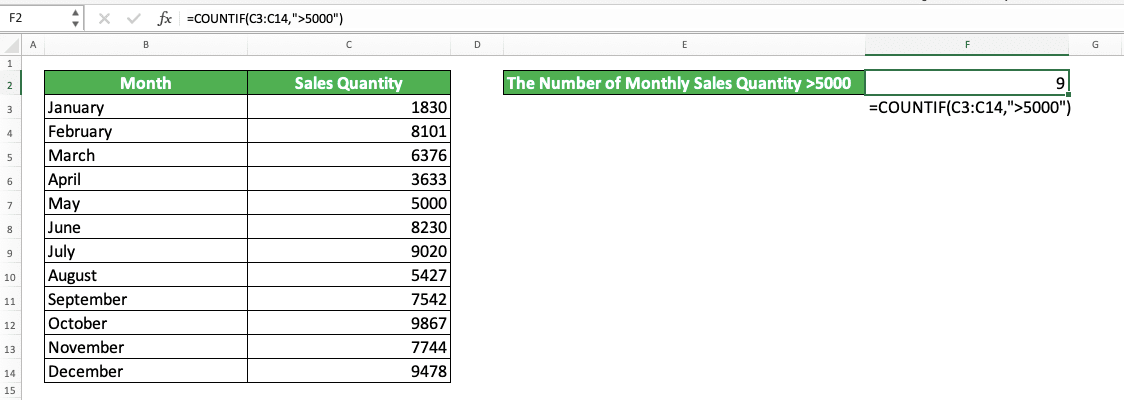



In this example, we can see the COUNTIF writing and final result. We use a cell range where all the sales quantity data is as the place to count the data.



The criterion we use to count the data is the sales quantity that is more than 5000. Because of that, we write “>5000” for the criterion input in the COUNTIF.

Input the cell range and criterion correctly based on your data processing needs. You will get your data counting result immediately!

Criterion Writing in COUNTIF

COUNTIF can accept many different kinds of writing for its criterion. The criterion you must write, of course, depends on what kind of data counting needs you have.

To give an illustration to you about what kind of criterion we might write in COUNTIF, here is its complete explanation. We divide the explanation based on the type of data that can be COUNTIF’s criterion.

Text (not case-sensitive)

Criterion Example	Explanation
"Jim"	The same as “Jim”
“<>Jim”	Not the same as “Jim”
“Jim*”	With “Jim” prefix
“*jim”	With “jim” suffix
“J*m”	“J” prefix and “m” suffix
“Jim?”	“Jim” prefix with any one character suffix
“?jim”	Any one character prefix with “jim” suffix
“J?m”	“J” prefix, any one character, and “m” suffix
“Jim~*”	The same as “Jim*”
“Jim~?”	The same as “Jim?”

A bit explanation of the symbols we can use for the text criterion:

• * = represents any character with any amount
• ? = represents any one character
• ~ = use this when you want to add * or ? character for the criterion

Number

Criterion Example	Explanation
70	Equal to 70
“>70”	More than 70
“<70”	Less than 70
“>=70”	More than or equal to 70
“<=70”	Less than or equal to 70

Date

Criterion Example	Explanation
“>”&DATE(2019,12,3)	Later than 3 December 2019

We don’t recommend inputting a date criterion using direct typing (e.g. “>3-12-2019”). The reason is that it can make your COUNTIF produces a wrong and unexpected result.

Cell coordinate

Criterion Example	Explanation
“>”&B1	More than the value in B1

Empty/non-empty cell

Criterion Example	Explanation
“"	Empty
“<>"	Not empty

Writing Steps

The following will explain the steps to write COUNTIF in excel.

We will explain these steps with their examples in screenshots to help you understand them easier.

1. Type an equal sign ( = ) in the cell where you want to put the data counting result
   
   
   
   
2. Type COUNTIF (can be with large and small letters) and open bracket sign after =
   
   
   
   
3. Input the cell range where you want to count data based on your criterion. Then, type a comma sign ( , )
   
   
   
   
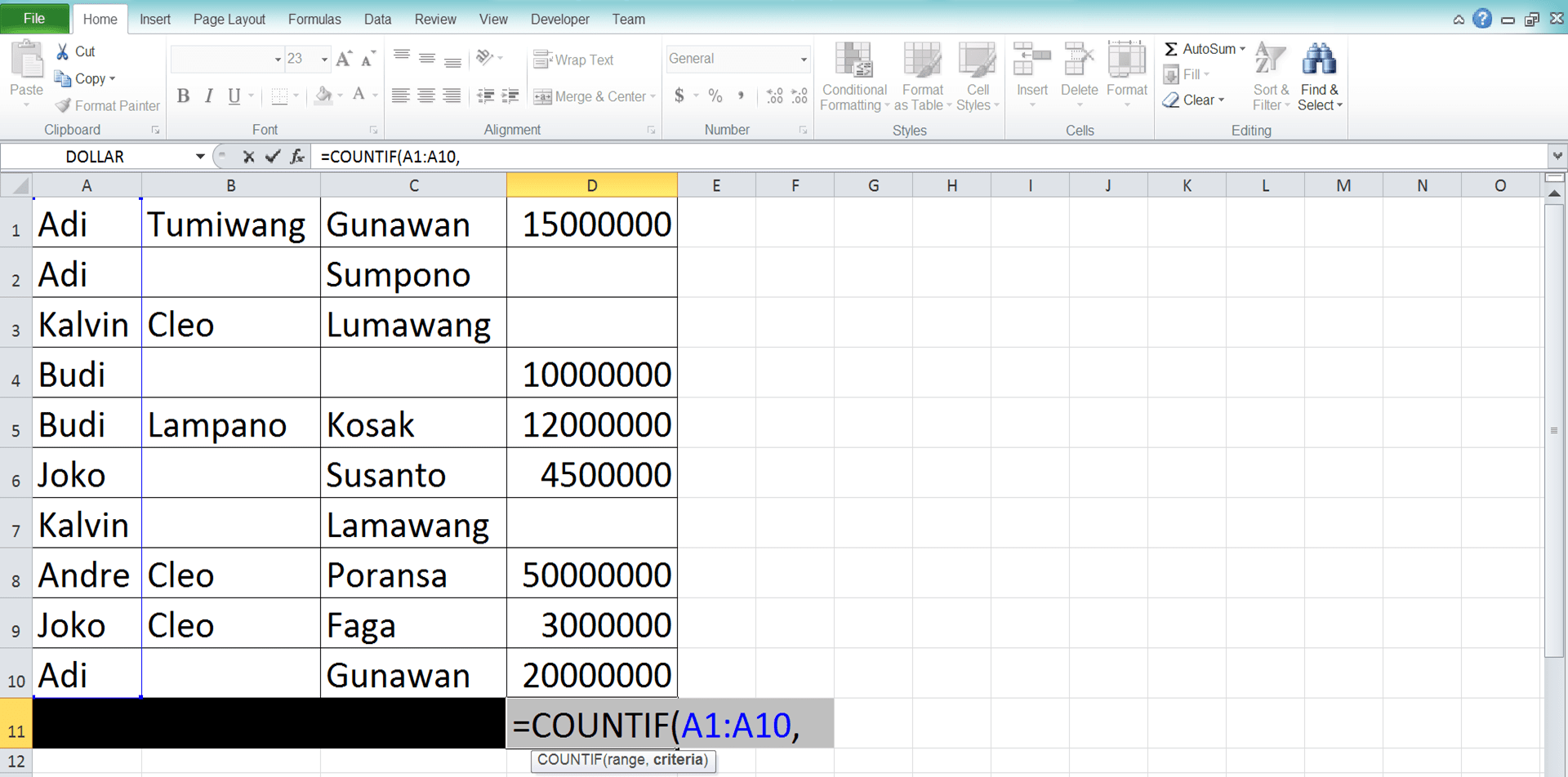
4. Input your data criterion
   
   
   
   
5. Type a close bracket sign
   
   
   
   
6. Type Enter
7. Done!
   
   
   
   

Main Reasons Why Your COUNTIF Produces an Error/Wrong Result

Finding it difficult to get the correct result from your COUNTIF? This sometimes can happen and the reasons can be many.



However, based on our experience, several factors can become the main reasons for an error/wrong COUNTIF result. Those factors are.

• Wrong criterion writing. This factor usually becomes the main reason why COUNTIF produces an error/wrong result. Make sure the criterion you input is a legit one
• Trying to input more than one criterion into COUNTIF. If you need to count data that meets more than one criterion, use COUNTIFS. The explanation of how to use this formula is in the next part of this tutorial
• Inputting the wrong cell range. Try to check your cell range input again. Have all the places where you want to count your data are already in this cell range?

Make sure you don’t do them as they can cause your COUNTIF to produce an error/wrong result!

COUNTIF With OR Criteria

Have you ever used the OR formula in excel?

OR is a formula that can help to evaluate more than one logic condition/value in excel. If at least one of them is right/TRUE, then it will give a TRUE result.

What if we want to do something like that when counting data using COUNTIF? We have more than one criterion to count our data. Moreover, we want COUNTIF to count all the data that fulfill at least one of those criteria.

Can we do that?

Of course, we can. Not by using OR in COUNTIF, but by summing all the COUNTIFs which number is based on your number of criteria. We use each COUNTIF to count data for 1 criterion. Thus, you will count the amount of data that fulfill at least one of your criteria.

Generally, here is the COUNTIF writing form by using the principle similar to OR.



If you use 2 criteria, then sum 2 COUNTIFs. If 3, then sum 3 COUNTIFs, and so on. The cell range you input in those COUNTIFs should be the same. This assumes that the data you want to count with all your criteria are in the same place.

To make it clearer about this COUNTIF implementation with the OR principle, here is its example in excel.



Here, we want to count the number of monthly sales quantity which is more than 7000 or less than 3000. We do it by using the COUNTIF sum method, just as you see in the formula writing.

We input each “or” criterion in each COUNTIF with the same cell range input (the sales quantity column). That means one COUNTIF for the “>7000” criterion and one more COUNTIF for the “<3000”.

Sum those two COUNTIFS and we will get the result we want! We will immediately know the number of sales quantity which is more than 7000 or less than 3000.

COUNTIF With AND Criteria: COUNTIFS

What if we need to count data that fulfill our criteria based on an AND principle? That means we only need to count data that fulfill all the criteria we have.

For this, we better not use COUNTIF. It will be much easier if we use its sibling formula, which is COUNTIFS.

The function of the COUNTIFS formula itself is similar to what we need here. It can help us count the amount of data that meet one or more specific criterion. By using COUNTIFS, we can do COUNTIF with the principle similar to AND!

Here is the general form of COUNTIFS writing.



In COUNTIFS, we input cell ranges and criteria continuously until we have inputted all our criteria. Each criterion input in COUNTIFS will evaluate its cell range pair only.

We can input the same or different cell range for each criterion depending on our data counting needs. If using different cell ranges, make sure all the cell ranges are inline and have the same size.

To understand better about COUNTIFS implementation, here is the example in excel.



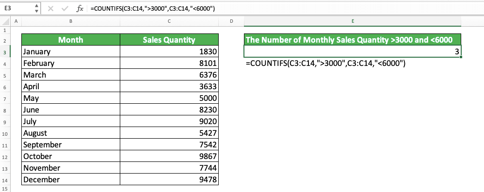
Here, we use COUNTIFS to count the number of sales quantity which is above 3000 and less than 6000. For that, we input the sales quantity cell range twice with each of the criteria input after the cell range input.

COUNTIFS will count the amount of data that fulfills all the criteria we input in it. If it doesn’t meet even one criterion, then COUNTIFS won’t count it.

In the example, we can see the amount of data that fulfill the two criteria we have is 3. This is because there are only 3 monthly sales quantities there that fulfill those two criteria (April, May, and August).

COUNTIF to Count Duplicates

Want to count how many duplicates you have in a cell range? You can do that by using COUNTIF.

How do we use COUNTIF in this case? First, you need to create a helper cell range that identifies the duplicates in your data cell range. After that, you count the identifiers given in that helper cell range by using COUNTIF to get the number of duplicates!



As an example, let’s say we have a name data column like this.



We can see there are some duplicates there. How to count how many of these duplicates are there in the name data column?

First, we make a helper column for the COUNTIF as explained previously to identify the duplicates. For the example of the name data column, the helper column and its contents will look like this.



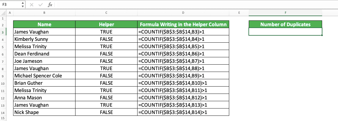
The “Formula Writing in the Helper Column” column is only there to help you see the formula in the helper column (you don’t need to use a column like that when you count duplicates in your excel).

We use COUNTIF too to identify the duplicates. In the example, we can see how we write the COUNTIF for the identification.

We can explain the process in the COUNTIF formula like this. We input the name column cell range and the name which is parallel with the helper column’s cell as its criterion.

We use $ symbols in the cell range input so it won’t move when we copy the formula (In this example, we write the formula in the helper’s column once for the data in the most top row. After that, we copy the formula down to get our results much faster).

If there is a duplicate for the data in the name column, then the COUNTIF result must be more than 1. Because of that, we input “>1” outside the COUNTIF to check that and produce a TRUE/FALSE logic value. If TRUE, then there is a duplicate for the data and if FALSE, then there isn’t.

We do this for all the names in the name column. With the TRUE/FALSE result, we will know whether there is a duplicate on the data or not. We can also count the amount of those duplicates by implementing COUNTIF to count data on the helper’s column.



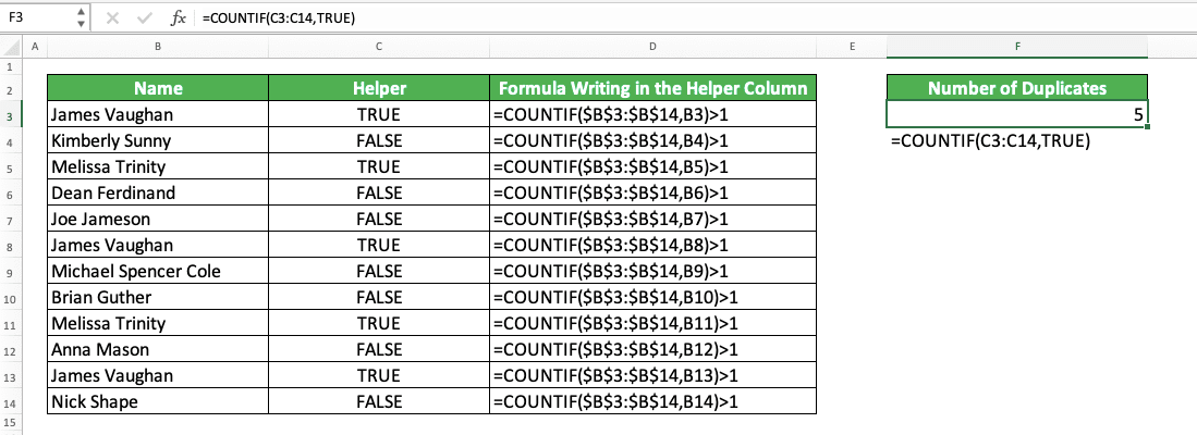
The COUNTIF criterion which counts all the duplicates is TRUE (because the identifier of the duplicates in the helper column is this TRUE value).

By doing all that, we can get the duplicates in our cell range quite easily!

COUNTIF to Count Unique Data

What if we want to count the amount of unique data in a cell range using COUNTIF? The way to do this is quite similar with the way to count the duplicates. However, we need to modify the formula in the helper column so we can use it to count the unique data.

To make this clearer, pay attention to this example. Let’s use the same name column with the one we use as the example to count duplicates earlier.



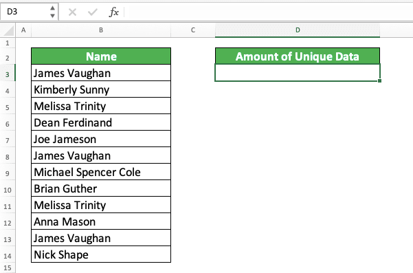
How to count the unique data in the name column? First, we make a helper column to help us count. Then, we fill this column with COUNTIF formulas like this.



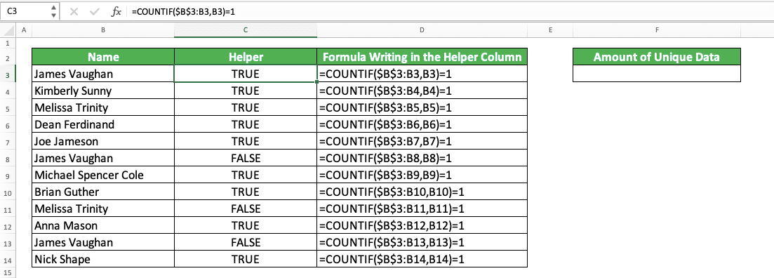
To count unique data, we use a cell range input that knows the last cell where we have counted the name. We do this so we can identify unique data from the duplicates in the name column (the data which has duplicates in the name column is counted as 1, however many the duplicates it has)

We input the cell range which follows the counting process by using $ symbols in the early cell of the cell range. We don’t give $ symbols in the later cell of the cell range so it can follow our counting process.

For the TRUE/FALSE requirement of the COUNTIF in the helper column, we use “=1”. This is because the unique data will make COUNTIF produces 1 as its result (If duplicates, then COUNTIF will produce 2, 3, and so on. This is because there are already more than one of the duplicates name in the cell range input).

The COUNTIFs in the helper column make us able to identify the unique data by looking at their TRUE/FALSE results. To count the unique data, we just need to count how many TRUEs are there in the helper column using COUNTIF.



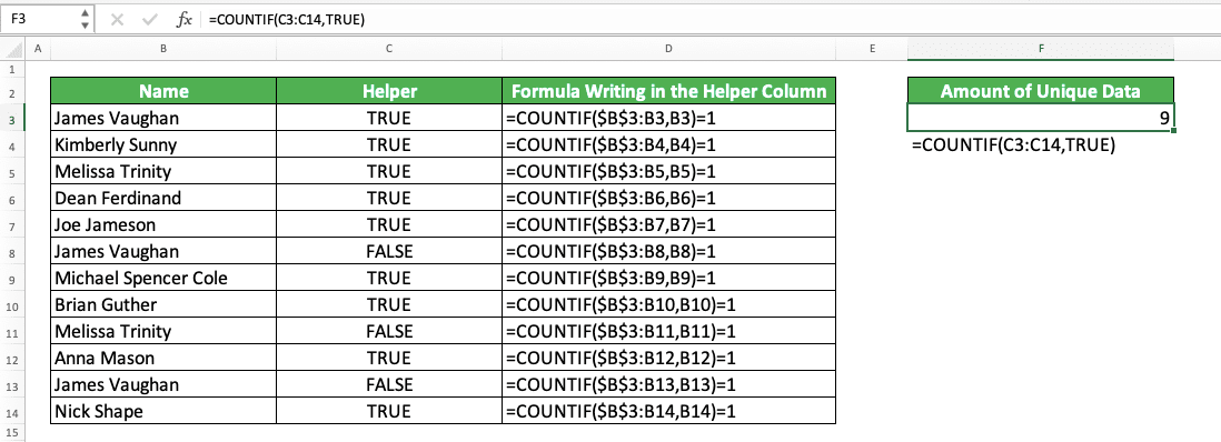
From there, we get the amount of unique data in the name column! Do it like this when you want to count the unique data in your excel.

Exercise

After you have learned how to use the COUNTIF formula in excel, let’s do an exercise. This is so you can deepen your understanding of the formula.

Download the exercise file and answer all the questions. Download the answer key file if you have done all the questions and want to check your answers. Or probably when you are confused about how to answer the questions!

Link to the exercise file:
Download here

Questions

Use the COUNTIF formula to answer the questions below:

1. How many times “Adi” shows up in the first column?
2. How many empty cells in the second column?
3. How many number data in the third column?

Link to the answer key file:
Download here

Additional Note

• COUNTIF isn’t case-sensitive when doing its data counting process
• If you use a text criterion in COUNTIF, then the maximum number of characters in it is 255 characters
• We cannot use COUNTIF to count data in a different workbook if the workbook is closed

Related tutorials you should learn: