How to Freeze Panes in Excel


In this tutorial, you will learn completely how to freeze panes in excel.
As we keep inputting and processing data, our data table in excel might get bigger and bigger. It may come to a point where it is troublesome to scroll around the data table to look at its content.
We may, for example, need to look at our table headers constantly. However, we need to keep going back and forth at the table to do that because of the large table size.
That is when the excel freeze panes feature can come to help with the situation. Want to know more about this feature and how to freeze panes optimally in excel? Read this tutorial until the end!
Disclaimer: This post may contain affiliate links from which we earn commission from qualifying purchases/actions at no additional cost for you. Learn more
Want to work faster and easier in Excel? Install and use Excel add-ins! Read this article to know the best Excel add-ins to use according to us!
Table of Contents:
- What is freeze panes?
- Freeze panes function
- How to freeze panes in excel: step-by-step
- How to freeze the top row in excel
- How to freeze the first column in excel
- How to freeze multiple rows in excel
- How to freeze multiple columns in excel
- How to freeze rows and columns simultaneously/freeze cells in excel
- Excel freeze panes not working? Possible reasons & solutions
- How to unfreeze panes in excel
- How to freeze cells besides top rows and most left columns
- Exercise
- Additional note
What is Freeze Panes?
Freeze panes is a feature that excel provides to “freeze” rows and/or columns in our worksheet. This is so they can stay viewable to us wherever we scroll.Freeze Panes Function
We can use freeze panes to make rows and/or columns stick in our view wherever we go in a worksheet. Usually, we utilize this function to keep viewing the row/column headers of our data table in excel.How to Freeze Panes in Excel: Step-by-Step
Here are the steps to use freeze panes in excel. They are quite simple once you get used to utilizing the feature.We explain the steps with example screenshots to make you understand them easier.
-
Place your cell cursor one cell outside the rows and columns you want to freeze (e.g. to freeze the two most top rows and three most left columns, place your cell cursor on cell D3)
-
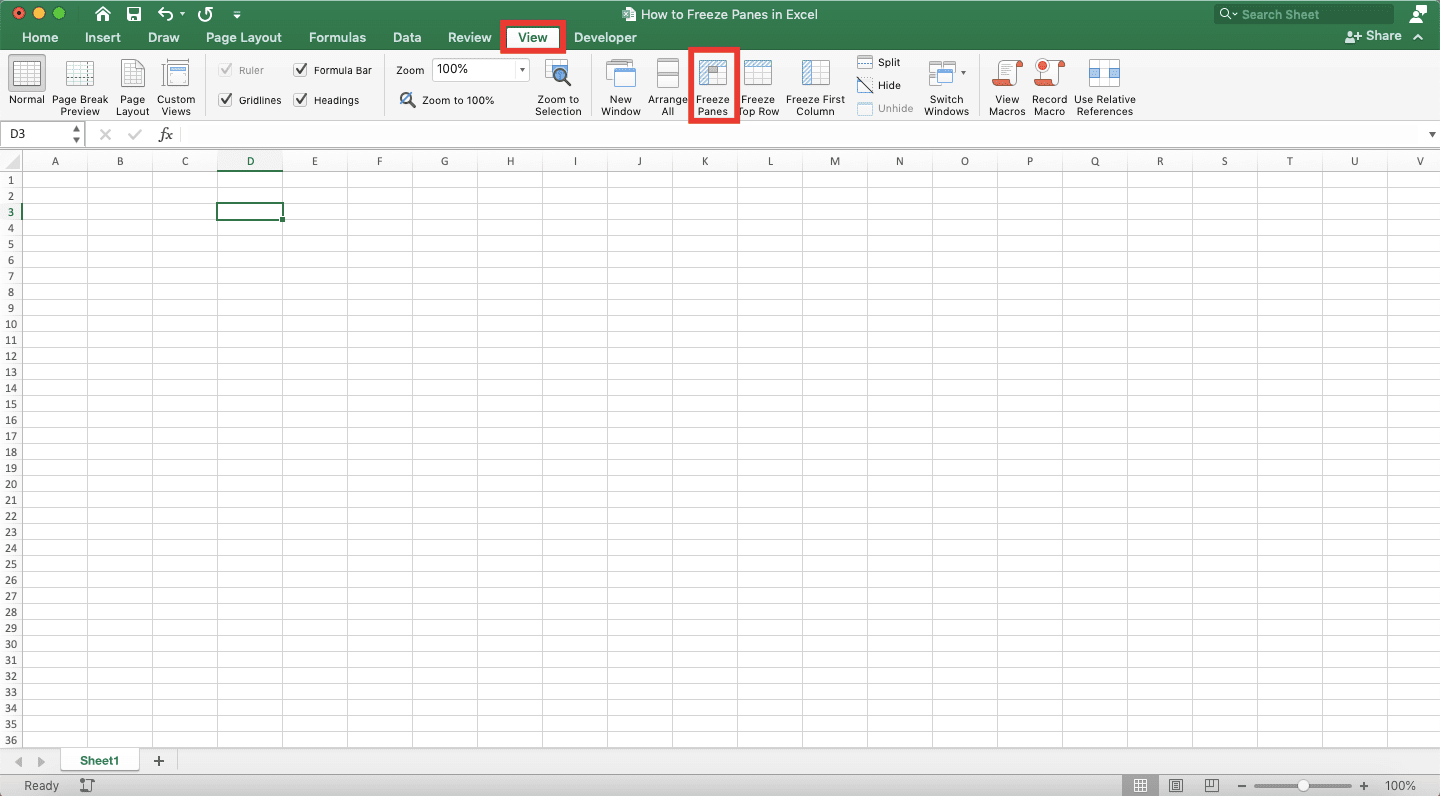
Go to the View Tab and click the Freeze Panes button there
-
Done! Now the rows and columns you freeze will always be viewable wherever you scroll on the worksheet

How to Freeze the Top Row in Excel
If you have understood the explanation earlier, then you might know now how to freeze the top row in excel.First, place your cell cursor in the A2 cell or highlight the second row of your worksheet. Then, click the Freeze Panes button in the View tab. To make it simpler, you can also just click the Freeze Top Row button in the View tab

Do any of the two methods and the top row of your worksheet will be viewable anywhere you scroll!
How to Freeze the First Column in Excel
To freeze the first (most left) column in excel, just place your cell cursor in B1 or highlight the second column. Then, click the Freeze Panes button. Alternatively, you can also click the Freeze First Column button in the View tab.
Do that and excel will lock the view of the most left column of your worksheet!
How to Freeze Multiple Rows in Excel
If you want to freeze multiple rows in excel, then place your cell cursor in the A column. Place it one row below the most bottom row you want to freeze. Alternatively, you can also highlight the row below that most bottom row.After that, click the Freeze Panes button in the View tab. You have frozen multiple rows now, which are viewable wherever you scroll in your worksheet.
How to Freeze Multiple Columns in Excel
The way to freeze multiple columns in excel is quite similar to freezing multiple rows, only this time is for columns.Place your cell cursor in the first row, one column right next to the most right column you want to freeze. Alternatively, you can highlight the column right next to that most right column.
After that, click the Freeze Panes button in the View tab. Doing that will freeze the multiple columns you want to still view anywhere you scroll in the worksheet!
How to Freeze Rows and Columns Simultaneously/Freeze Cells in Excel
What if you want to freeze rows and columns at the same time? If you have read the step-by-step instructions of how to freeze panes earlier, then you may have some idea.First, place your cell cursor just one cell outside the rows and columns you want to freeze. For example, if you want to freeze five rows and two columns, then place your cell cursor on cell C6.
Then, just go to the View tab and click the Freeze Panes button. You have frozen the rows and columns you want!
Excel Freeze Panes Not Working? Possible Reasons and Solutions
The freeze panes feature doesn’t work the way you want it to? There can be several possible reasons for that. However, these are probably the most possible ones.-
Reason: You place your cell cursor in the wrong place before you click the Freeze Panes button. Or you may highlight the wrong row or column. This can cause freeze panes to freeze the wrong rows and/or columns for you.
Solution: Make sure your cell cursor/highlighted column/row is just outside the rows and/or columns you want to freeze. Then, try to click the Freeze Panes button again. -
Reason: You don’t want to freeze the top rows and/or the most left columns of your worksheet. You want to freeze other rows/columns/cells instead. However, unfortunately, freeze panes cannot do this kind of action for you.
Solution: Use the method we will discuss later in this tutorial (split view). -
Reason: You cannot click the Freeze Panes button in the View tab. This can happen when you are in the edit mode of your cell or when your worksheet is protected.
Solution: Get out of the cell edit mode by pressing the Esc button and try to unprotect your worksheet.
Go through these three points and your freeze panes should work the way you want after that!
How to Unfreeze Panes in Excel
Have done freezing your rows and/or columns and you want to unfreeze them now? You can do that easily in excel.Just go to the View tab. Then, click the Unfreeze Panes button, which location is where your Freeze Panes button is previously.

Do that and you will unfreeze the rows and/or columns in your worksheet.
How to Freeze Cells Besides Top Rows and Most Left Columns
What if you want to make other cells besides top rows and most left columns viewable wherever you scroll? Can we do that using freeze panes?Unfortunately, freeze panes can only freeze top rows and most left columns in your worksheet. However, you can imitate what you want to do by using the Split button in the View tab.

Just click the button and your worksheet display will divide itself into four sections. When you scroll one section, the other will stay in their place and be viewable. That way, it can be similar to you freeze the cells in those other sections!

If you have done freezing your cells, then just click the Split button again to return to the normal view.
Exercise
After learning how to freeze panes in excel, you can practice your understanding by doing the following exercise!Download the exercise file from the following link and do the instruction below. Download the answer key file if you have done the exercise and want to check your answer!
Link to the exercise file:
Download here
Instruction:
Lock the black colored parts of the three sheets! Test by doing scroll on the three sheetsLink to the answer key file:
Download here
Additional Note
If you use Windows OS, then you can use a shortcut to freeze/unfreeze panes in excel. The shortcut is by pressing Alt + W and then F and then F.Related tutorials you should learn: