How to Use MAX IF Excel Formula: Usability, Example, and Writing Steps
Home >> Excel Tutorials from Compute Expert >> Excel Formulas List >> How to Use MAX IF Excel Formula: Usability, Example, and Writing Steps
In this tutorial, you will learn how to use MAX IF excel formulas combination. MAX IF can be used to find the largest value from numbers in which data entries fulfill specific criteria.
Disclaimer: This post may contain affiliate links from which we earn commission from qualifying purchases/actions at no additional cost for you. Learn more
Want to work faster and easier in Excel? Install and use Excel add-ins! Read this article to know the best Excel add-ins to use according to us!
Table of Contents:
- MAX IF usefulness
- MAX IF result
- The excel version since which the combination of MAX IF formulas can be used
- How to write MAX IF and its inputs
- The example of usage and result
- Writing steps
- Alternative: SUMPRODUCT MAX
- Looking for the n-th largest value with specific criteria: LARGE IF (or SUMPRODUCT LARGE)
- Exercise
- Additional note
MAX IF Usefulness
The MAX IF formula is useful if you want to find the largest value from all numbers that fulfill specific criteria.MAX IF Result
The result of MAX IF is the number with the largest value from numbers in which data entries fulfill specific criteria.The Excel Version Since Which the Combination of MAX IF Formulas Can Be Used
The MAX and IF formulas can be used since excel 2003.How to Write MAX IF and Its Inputs
Generally, the way to write the combination of MAX and IF can be illustrated as follows:
{=MAX(IF(criteria_range=criteria[…],number_range))}
The inputs used in the MAX IF writing can be explained as follows:
- criteria_range = the cell range contains data that you want to evaluate with your criterion
- criteria = the criterion you want to use to filter the numbers that will be compared to get your largest value
- […] = optional. The additional cell range and criterion pairs if needed. You should write additional IF formulas or multiply all the criteria cell ranges
- number_range = The cell range where the numbers which data fulfill your criteria are taken to be compared for the largest value
Maybe you realize there are curly bracket signs ( {} ) that envelops the formula. This sign means that the formula is an array formula.
The array form is needed here because we will use IF to evaluate data in cell ranges. When we use excel formulas that usually have one data input to process data in ranges, an array formula is needed.
This array formula can be activated in excel by pressing the Ctrl + Shift + Enter buttons (Command + Enter on Mac for the excel version before 2016 and Control + Shift + Enter for the excel version 2016 and after) simultaneously after finishing the formula writing.
Another thing to remember for the MAX IF cell ranges inputs is all of them must have the same size. Moreover, they should be in line with each other so it is easy if you want to check the result logic.
The example of Usage and Result
The following will give and explain the usage and result example of MAX IF in excel.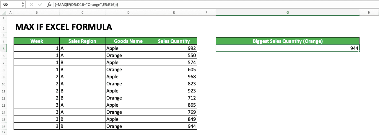
In the example above, we can see how to use the MAX IF formula with one criterion. As illustrated in the previous part, the IF formula needs to be inputted into your MAX formula.
The inputs of the IF itself are the cell range for the criterion evaluation, the criterion, and the numbers cell range. The = sign between the cell range and its criterion represents the relationship symbol that becomes the base of the evaluation process.
In the example, we want to get the largest sales quantity from data entries with the “Orange” goods name. For that, we input the “goods name” cell range with “Orange” as its criterion, connected with the = sign.
The combination of MAX IF formulas is an array formula because we evaluate data in cell ranges in our IF. In the formula process, each data in the criterion cell range will be evaluated by the criterion.
From this evaluation, our IF will produce the TRUE/FALSE logic value for each data entry. For the example above, the comparison result between the criterion and the cell range is approximately like this:
(FALSE, TRUE, FALSE, TRUE, FALSE, TRUE, FALSE, TRUE, FALSE, TRUE, FALSE, TRUE)
Each entry with the “Apple” goods name will become FALSE and each entry with the “Orange” goods name will become TRUE (because the goods name criterion is “Orange”). From the comparison result, the numbers from the data entries with the TRUE result will be compared by MAX.
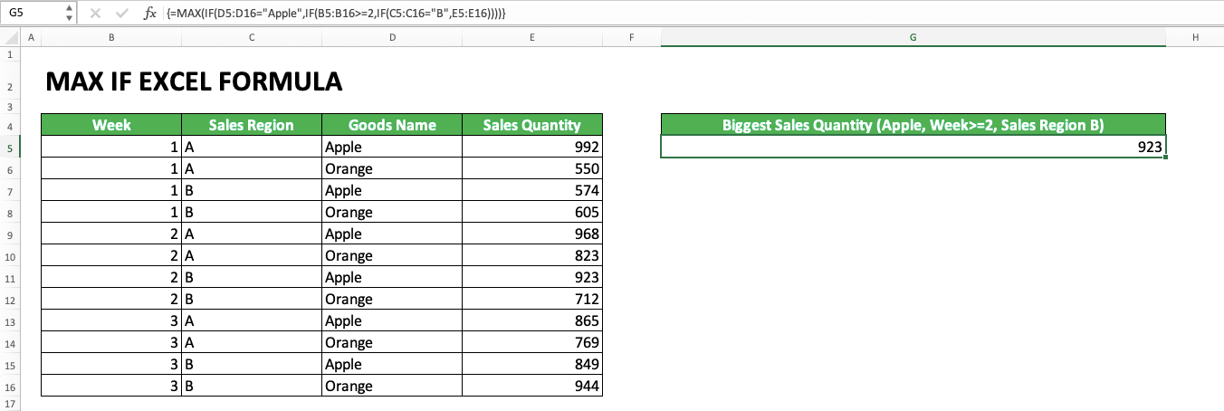
The next example is the MAX IF formula writing with more than one criteria. Here, the criteria are “Apple” goods name, week more than or equal to 2, and sales region B. Only the data that fulfill all the criteria, produce TRUE for all of them, will be compared their numbers by MAX.
To input more than one criteria in the MAX IF, you need to use IFs as many as your criteria.
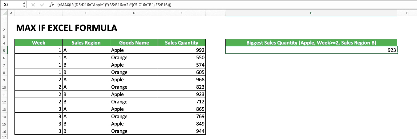
In the third example, we can see the alternative for the MAX IF formula writing with more than one criteria. You can also input the cell ranges and criteria pairs by multiplying them all in your IF.
Because TRUE is 1 and FALSE 0 in excel, then the multiplication will eliminate the data entries which have FALSE. In other words, we will get filtered data entries for their numbers to be compared by MAX.
After writing your MAX IF formula with whichever writing style used above, don’t forget to press Ctrl + Shift + Enter. Those three buttons will change your formula to an array formula. If you just press Enter after writing the MAX IF formula, then the formula won’t function well.
Writing Steps
Here is the detailed explanation of the step-by-step writing of the MAX IF excel formula. Each step will be accompanied by a screenshot to help your learning process.-
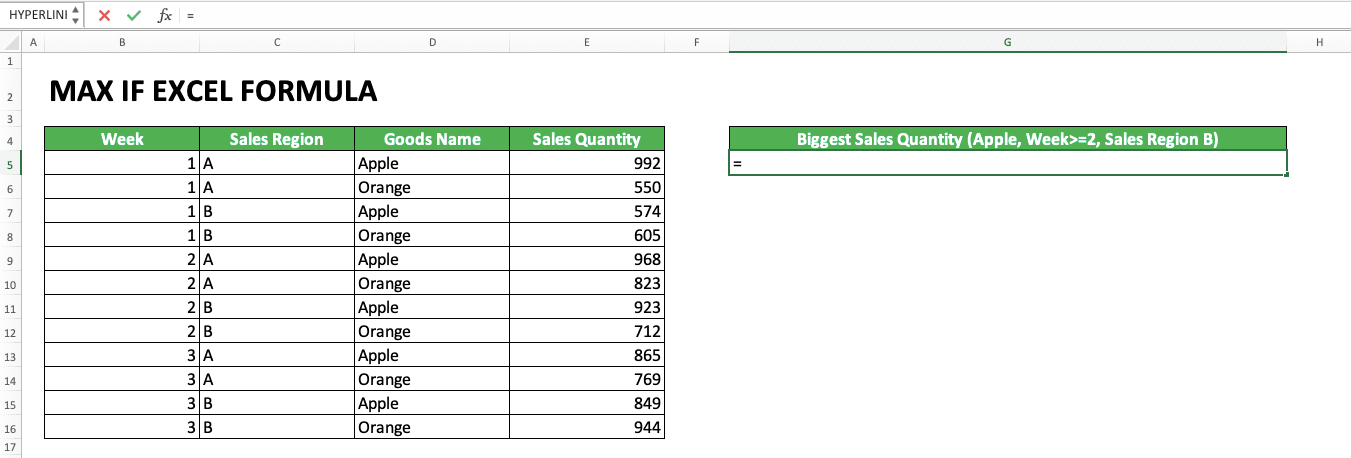
Type an equal sign ( = ) in the cell where you want to put in your MAX IF result
-
Type MAX (can be with large and small letters) and input an open bracket sign

-
Type IF (can be with large and small letters) and input an open bracket sign

-
Input the cell range where the data you want to evaluate with your criterion is. Then, input an equal sign ( = ) or other signs which represent the data evaluation process in this cell range by your criterion

-
Input the criterion you want to use to evaluate the data in your previously inputted cell range
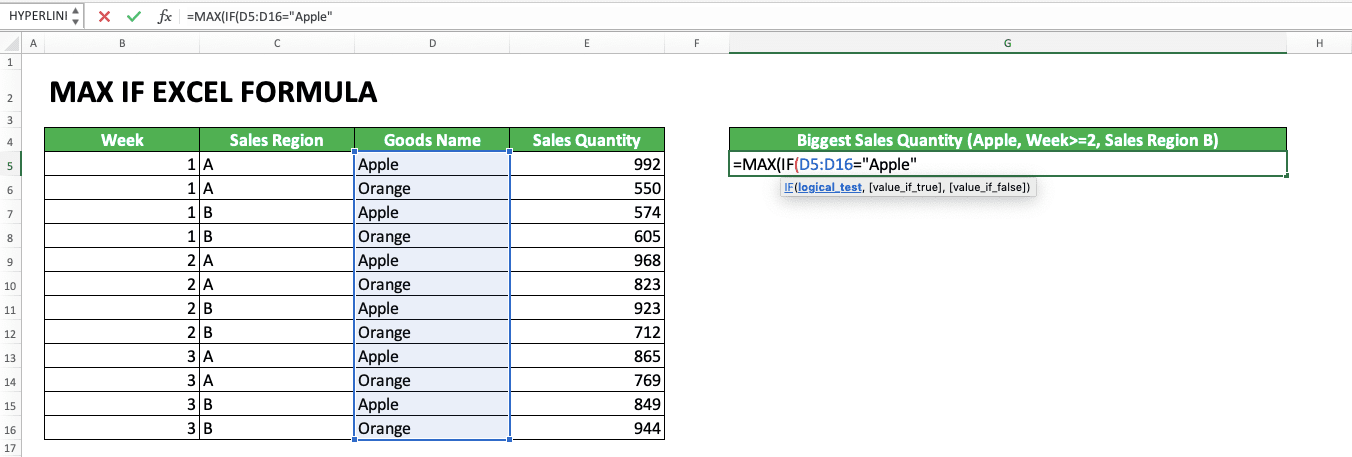
-
Optional: Input other cell range and criterion pairs if needed. There are two ways to input these additional pairs of cell range and criterion:
- First method: Input a comma sign ( , ) then repeat steps 3 to 5. Repeat the input of comma sign and steps 3-5 until all your cell range and criterion pairs have been inputted
- Second method: Make a bracket sign which envelops the inputs from step 4 to 5. Then, input a star sign ( * ) then repeat the bracket sign input and steps 4 and 5. Repeat the inputs of star sign, bracket sign, and step 4-5 until all your criteria have been inputted


-
Input a comma sign and the cell range where the numbers which will be compared to get the largest value are. Later, only the numbers which are in line with the data that pass your criteria will be taken for the comparison

-
Input close bracket signs with the numbers needed (depending on the open bracket signs that haven’t been closed in this MAX IF formula writing of yours)

- Press the Ctrl + Shift + Enter buttons (On Mac, Command + Enter for the excel version earlier than 2016 and Control + Shift + Enter in the excel version 2016 afterward) simultaneously
-
The process is done!

Alternative: SUMPRODUCT MAX
If you don’t want to use an array formula to get the biggest value that fits your criteria, use SUMPRODUCT MAX. An example of this formula combination writing can be seen in the screenshot below.
By using SUMPRODUCT MAX, you don’t need to use an array formula to get your biggest value. The result produced by SUMPRODUCT MAX is similar to the MAX IF result as you can see below.
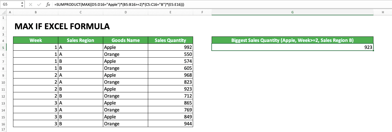
The SUMPRODUCT MAX method can succeed because the SUMPRODUCT function multiplies in matrix the numbers between all its cell ranges input. Because TRUE is 1 and FALSE is 0 in excel, SUMPRODUCT will automatically eliminate all data entries that have FALSE. As we know, anything that is multiplied by 0 will become 0 too.
Looking for the N-th Largest Value with Specific Criteria: LARGE IF (or SUMPRODUCT LARGE)
If what you need is the second or third or other nth largest number, then use LARGE IF. The way to use LARGE IF is similar to MAX IF. It is just you need to add the descending order input of the number you want to get from LARGE.
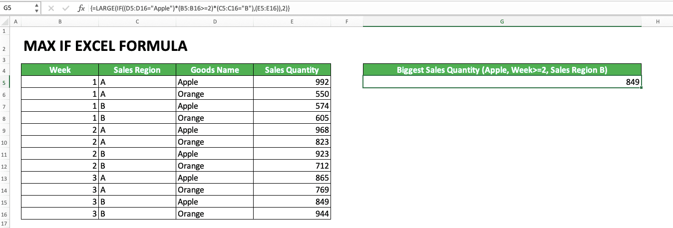
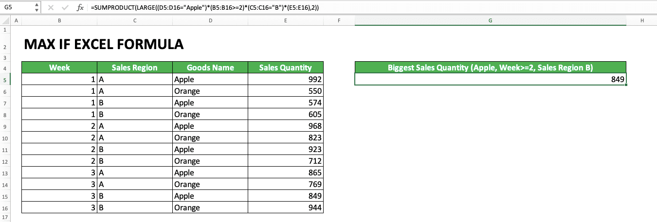
Like the MAX IF, you can also utilize SUMPRODUCT as the alternative to LARGE IF. The way to write SUMPRODUCT LARGE is similar to SUMPRODUCT MAX. Don’t forget to add the descending order input of the largest number you want to get when you use SUMPRODUCT LARGE.

Exercise
After learning how to use MAX IF, now is the time to practice your understanding through this exercise!Download the exercise file and answer all the questions. Download the answer key file if you have done the exercise and want to check your answers!
Link to the exercise file:
Download here
Questions
Answer in the appropriate gray-colored cells!- What is the largest average score from the eleventh and twelfth class for all subjects? Use MAX IF to answer this question!
- What is the largest average score from the tenth and eleventh class in the Biology subject? Use MAX IF to answer this question!
- Use SUMPRODUCT MAX to answer question number 2!
Link to the answer key file:
Download here
Additional Note
- If you want the smallest number with specific criteria, then you just need to change MAX to MIN in your writing. The way to use MIN IF is almost the same as MAX IF which has been explained in this tutorial (or use SUMPRODUCT MIN if you don’t want to use an array formula)
- If you want the nth smallest number with specific criteria, then just change the LARGE formula to SMALL. The way to use SMALL IF is almost the same as LARGE IF which has been explained previously (or use SUMPRODUCT SMALL if you don’t want to use an array formula)
- If you have excel version 2019 or above, then you can use the MAXIFS formula for an easier way (don’t need to combine MAX and IF). MAXIFS has the same function as the MAX IF formulas combination
Related tutorials you should learn too:


