Multiplication in Excel and All Its Formulas & Functions

In this tutorial, we will discuss various ways to do multiplication in excel. Besides how to write the formula manually, we will also talk about the use of PRODUCT and paste special to multiply.

If you haven’t understood how to do this calculation in excel, then you have come to the right place! After finish learning all the materials here, you should be able to do excel multiplication easily.

Disclaimer: This post may contain affiliate links from which we earn commission from qualifying purchases/actions at no additional cost for you. Learn more

Want to work faster and easier in Excel? Install and use Excel add-ins! Read this article to know the best Excel add-ins to use according to us!

How to Multiply Numbers in Excel

If you want to learn multiplication in excel, then the first thing you should learn is the way to multiply numbers.

The process to do numbers multiplication in excel itself is pretty easy. You just need to type a standard multiplication formula in your cell with star signs (*) as the multiplication symbol. Of course, you should type an equal sign ( = ) first as the symbol of formula writing in excel.

In general, here is the standard writing form of a multiplication formula in excel for numbers.



If there are more than two numbers you need to multiply, then add more star signs and numbers in your typing. The numbers in the formula can be typed directly or inputted through cell coordinates where the numbers are.

To make it clearer about numbers multiplication formula writing in excel, see the implementation example below.



As seen in the dollar multiplication example above, we can get a multiplication result using the writing form explained previously. We can see in the example’s formula bar, how to write a multiplication formula for all the numbers in the example.

Type an equal sign and input all the numbers you want to multiply. Don’t forget to add * signs between the numbers. After finish writing the formula, press enter. You will then get the multiplication result you need!

How to Multiply Percentages in Excel

The way to multiply percentages in excel is similar to how to multiply numbers. It is just, you need to make sure your percentages are in percentages, or at least in its decimal equivalent form. This is so you can get the correct result from your calculation.

Generally, here is the writing form of percentages multiplication formula in excel.



Almost the same as numbers multiplication, right? If your percentage number already has a % sign behind, then just write the formula like the one above. Or if using its decimal equivalent, then it should have the same value as the percentage number value divided by 100 (for example, 80% is equivalent to the 0.8 decimal, the result of 80 divided by 100).



The implementation example of the percentages multiplication formula in excel and its result is as follows.



Look at the example’s formula bar. The writing pattern is the same as numbers multiplication, right? Input the number to multiply, the * sign, and the percentage in one writing and enter. You will get the percentage multiplication result after that.

How to Multiply Columns in Excel

What if the numbers you want to multiply are spread per column and you want to multiply them fast?

Don’t worry because that means you just need to copy your multiplication formula after you write one. This is useful if there are many numbers in your columns and you need to multiply the numbers per row.

The way to write a formula in your column is the same as writing a normal numbers multiplication formula in excel.



You just need to add more numbers and star signs if you want to multiply more than two numbers.

As an example of the columns multiplication, see the following data.



In the example, we want to multiply per row all the numbers in column 1 to 3. How to do it? First, we type our multiplication formula in the first row of the column like this.



Then, we move our pointer to the bottom right of the cell cursor until it changes into a + sign like this.



Next, we just click and drag our pointer until the bottom of the row we want to multiply. Let go of the drag and it is done!



You have got the multiplication result of each row for all the columns’ numbers.

Multiplication in Excel With Constants

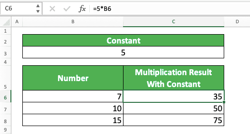
What if you have constants for all the numbers you want to multiply in excel? That means there is one particular number you want to multiply with all your other numbers. Do you need to write separate multiplication formulas for each of the multiplications?

You don’t have to. You can make one multiplication formula and copy it by making your constant cell as an absolute reference first. Or if not, you can also type directly the constant number in your multiplication formula so it doesn’t change when copied (not using a cell coordinate).

If you want to use an absolute reference for your constant cell, then you need to add $ signs. Add them in front of your constant cell coordinate’s column letter and row number. To add them, you can type them directly or press F4 (Command + T in Mac) once when your cursor is in the cell coordinate.

The general form of the constant multiplication writing itself is almost identical to a normal numbers multiplication.



To make you understand better, here is an example of constant multiplication formula writing. The example given is a constant multiplication writing with direct typing and an absolute cell coordinate reference.



Direct typing:



Absolute cell coordinate reference:



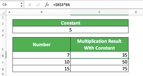
Easy, isn’t it? By typing directly or using an absolute cell coordinate reference, you just need to type your formula once. After done typing, copy the formula to other cells to get the other number and constant multiplication results!

How to Multiply Matrices in Excel

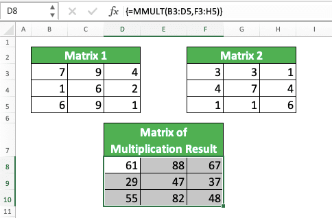
Sometimes, you also need to multiply the number matrices you have in excel. To do this kind of multiplication easily, you can utilize the excel MMULT function.

Generally, this is how we write MMULT in excel.



Why do we have curly brackets around the MMULT formula writing? Those are the symbol of an array formula form in excel!

We usually have our number matrices in the form of cell ranges in excel. To multiply those cell ranges and get our result in full, we should use the array formula form.

In the MMULT writing form itself, we input the cell ranges where we put our number matrices. To get the array formula form, we press Ctrl + Shift + Enter (Control + Shift + Enter in Mac) buttons after we finish writing the formula (we cannot type the curly brackets ourselves). By doing that, we can get our matrices multiplication result correctly!

To do the matrixes multiplication itself, first, we need to highlight the cell range where we want to put the result. To make the understanding easier, look at the example below when we highlight the cell range for our matrixes multiplication result.



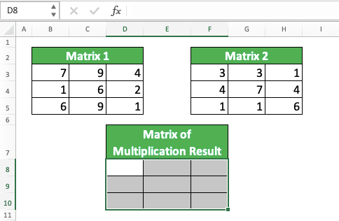
After highlighting the cell range, we type MMULT and input the matrix cell ranges we want to multiply. Press Ctrl + Shift + Enter after we finish with the MMULT formula writing and your matrixes multiplication result will be there!

How to Multiply and Sum (Or Other Relevant Operations) in Excel

What if we want to multiply and then sum or do other numbers processing at once? Can we do that or we must multiply our numbers first before processing them further?

By using array forms, we can multiply and do another process on all of our numbers at once. This can be done in one writing. Special for sum, we can also use SUMPRODUCT as an alternative method.

If you use SUMPRODUCT, then the writing form is like this.



If there are more than 2 cell ranges to multiply, you just need to add the cell ranges and * signs.

For a clearer explanation for this SUMPRODUCT, here is its implementation example.



In the example, we input cell ranges we want to multiply (quantity and price columns) to then sum the multiplication results.

We can do it in phases by knowing the multiplication results per row first before summing them. However, we can also do it directly using SUMPRODUCT.

In our formula, the numbers in the quantity and price cell ranges are multiplied first in SUMPRODUCT. Because our multiplication is a cell ranges multiplication, the result of the example becomes an array like this.



The numbers there are the multiplication result of the numbers that have the same position in the quantity and price columns (3x20000, 2x30000, 3x25000). After we get the array, SUMPRODUCT will sum all the numbers in it as per its function. From there, we get 195000, which becomes the number we put in the cell.

What if we want to use another way to multiply and sum? Or we want to multiply our numbers then do another operation like using MAX or AVERAGE formula?



The general array formula writing form to do that can be illustrated as follows.



Like SUMPRODUCT, if there are more than 2 cell ranges, then you just need to add the cell ranges and * signs. Make sure the formula you use accepts a number cell range as its input so this won’t produce an error.

As an example of this array formula implementation, take a look at the screenshot below.



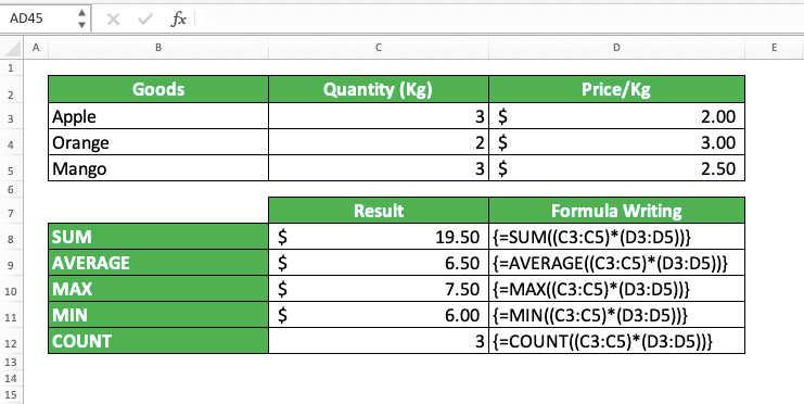
As shown in the example, we can use SUM, AVERAGE, MAX, MIN, and COUNT among the formulas combined with the multiplication. Multiply the cell ranges containing the numbers in the formula we use and press Ctrl + Shift + Enter. We will get the multiplication and the formula processing directly!

The array form becomes important here because the multiplication result in the formula we use is an array. Don’t forget to use that form because your formula will produce an error if you forget.

Alternative Multiplication Method 1: PRODUCT

What if we want to multiply many numbers in a particular cell range fast? It is troublesome if we need to write the multiplication formula with * signs because we need to input all the numbers. Is there another way we can use in that situation?

The answer to that question is there is another way. We can use the PRODUCT formula to make our formula writing much quicker to get the multiplication result we need.

How to use this formula? If you have used SUM before, then the usage principle of PRODUCT is similar. You just need to input the cell range which contains the numbers you want to multiply as its input.

Generally, here is the writing form of PRODUCT in excel.



Although officially, we can input many numbers/cell coordinates, we often only use one cell range input. However, if needed, you can also input more than one cell range/numbers/cell coordinates.

Here is an example of PRODUCT usage and result in excel.



The example of the PRODUCT writing can be seen in the formula bar. As shown there, we just need to input the cell range that contains our numbers in PRODUCT. This formula will then give the cell range’s numbers multiplication result directly.

If you want to learn further about PRODUCT, you can read this tutorial which discusses it specifically.

Alternative Multiplication Method 2: Paste Special

There is one more method to do multiplication in excel, which is by utilizing the paste special feature. By using this method, you can multiply your numbers without any need to write a formula.

To make it clearer, let’s see its implementation example. For paste special, first, you need to get the cell containing a number you want to multiply into a copy mode.

This mode can be activated by pressing Ctrl + C (Command + C in Mac) on the cell. It is already active if your cell has dotted lines move around it. You can see the example in this screenshot.



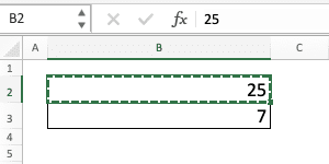
After those lines are there, move your cursor to another cell where you place the other number you want to multiply. Click the dropdown in the Paste menu on the Home tab and choose Paste Special…



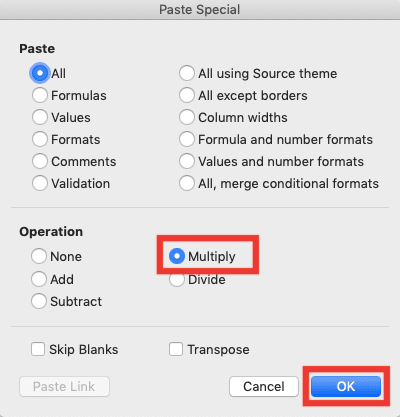
In the dialog box shown, choose Multiply in the Operation part. After that, click OK.



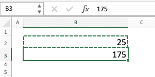
Your number has been multiplied in the cell where you do the paste special. You don’t need to write any formula to do it!

Exercise

After learning how to multiply in excel, now let’s do an exercise. We provide the exercise so you can deepen your understanding on what you have learned just now.

Download the exercise file and answer all the questions. Download the answer key file when you have answered all the questions. Or probably when you are confused about how to finish one or all the questions!

Link to the exercise file:
Download here

Questions

1. How much total payment is needed for hot dogs, hamburgers, and french fries? Use the manual method with the star sign ( * ) to answer!
2. How much total payment is needed for tacos and sandwiches? Use PRODUCT to answer it!
3. How much total payment is needed for all the food? Use an array formula form to answer it!

Link to the answer key file:
Download here

Additional Note

PRODUCT is seldomly used because you usually only need to multiply a few numbers. However, when you need to multiply many numbers, your understanding of PRODUCT will be very helpful.



Related tutorials you should learn: