CONCAT Excel Formula: Functions, Examples, and How to Use

In this Compute Expert tutorial, we will learn how to use the CONCAT excel formula completely. We can start using this formula since excel 2019 and excel office 365.

In the previous Excel versions, you may have known CONCATENATE as the formula to combine excel data into one text. CONCAT is the upgraded version of CONCATENATE as it can do some things that CONCATENATE can’t.

Curious to learn more about this CONCAT formula? Read this tutorial until its last part!

Disclaimer: This post may contain affiliate links from which we earn commission from qualifying purchases/actions at no additional cost for you. Learn more

Want to work faster and easier in Excel? Install and use Excel add-ins! Read this article to know the best Excel add-ins to use according to us!

CONCAT Function in Excel

We can use CONCAT to combine multiple data into one text.

CONCAT Result

The result we get from CONCAT is a text that contains all of the data you give as its inputs.

Excel Version from Which We Can Use CONCAT Excel Formula

We can start using CONCAT in excel since excel 2019.

The Way to Write It and Its Inputs

The general writing form of CONCAT in excel is as follows.



The data1, … input there is all the data you want to combine into one text using CONCAT. You can input them in the form of direct data typing, cell coordinates, or cell ranges.

If you give more than one input to CONCAT, then don’t forget to separate them using comma signs ( , ).

Example of Its Usage and Result

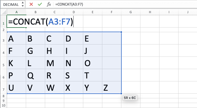
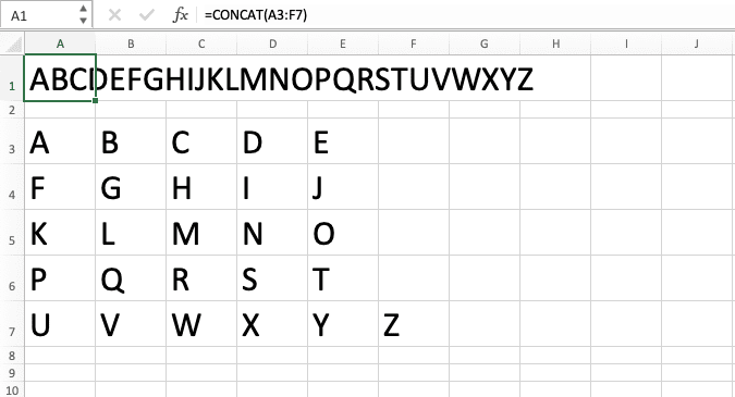
Here is an example of CONCAT implementation and result in excel.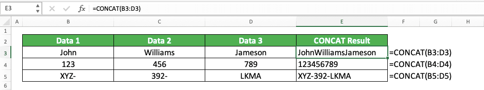



As you can see there, we use CONCAT to combine our data per row into one text. We just need to input the cell range where the data we want to combine are and CONCAT will combine them.

So simple, right? The capability to accept a cell range input is also an upgrade of CONCAT compared to CONCATENATE. If we use CONCATENATE, then it can only just accept direct data typing and/or cell coordinate inputs.

Writing Steps

After we have discussed the CONCAT writing form, inputs, and implementation example, now let’s discuss its writing steps. The steps to write CONCAT in excel are actually pretty simple, as you will see in the following.

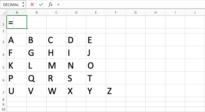
1. Type an equal sign ( = ) in the cell where you want to put the CONCAT result
   
   
   
   
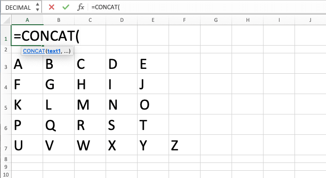
2. Type CONCAT (can be with large and small letters) and an open bracket sign after =
   
   
   
   
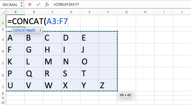
3. Input all the data/cell coordinates/cell ranges which data you want to combine into a text. Don’t forget to type comma signs ( , ) in between the inputs you give
   
   
   
   
4. Type a close bracket sign after you have inputted all the data you want to combine
   
   
   
   
5. Press Enter
6. Done!
   
   
   
   

Common Reasons Why CONCAT Produces an Error/Wrong Result

Getting an error/wrong result from your CONCAT and you are confused why that happens?

CONCAT, like any other formula in excel, can produce an error/wrong result if you use it incorrectly. There are many possible factors that can cause this unwanted result. However, the most probable factors might be:

• There are some unexpected values in your CONCAT inputs. The cells which look empty might contain some spaces or there can be data you don’t recognize in your cell range. Check your CONCAT again and see where the parts of its combined text result come from!
• There are error values within the data input you give to CONCAT. Any error value in your CONCAT inputs will make you get an error too from CONCAT!
• Expect separators like spaces or commas in your CONCAT result? Don’t forget that CONCAT only gives the combined result of your data without automatic separators. If you want to use separators, then input them manually or use the alternative method we discuss later in this tutorial!

Evaluate your CONCAT with those points above in mind if you get any wrong/error result!

CONCAT 2 Columns or More in Excel

If you have seen the CONCAT implementation example before, then you might have understood the way to use CONCAT for columns. You just need to input the data you want to combine in those columns to CONCAT.

As we usually combine our data per row in columns, then you just need to write CONCAT for the first row. Copy the CONCAT you write across those columns rows and you will get all the CONCAT results you need!

Here is one example of combining two columns data using CONCAT.



As discussed, we just need to input the row cell range of those columns which data we want to combine. After we write the CONCAT formula for the first row, copy it down to get all the column combination results.

However, if we need to have separators in our CONCAT results, then we need to input them manually. The separators’ inputs implementation in CONCAT for the above columns data is as follows.



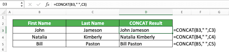
As we don’t have separators in our cell range input to CONCAT, we need to input the data using cell coordinates. Between the cell coordinates inputs, we type a space ( “ “ ) directly to CONCAT.

Do that for the first CONCAT writing, copy it down, and we will get all the CONCAT columns results we need!

CONCAT with Separators in Excel: TEXTJOIN

CONCAT can combine our data in a cell range fast and easily. But what if the cell range we want to combine the data from is large and we want separators?

Using CONCAT for this can be troublesome because we need to input the cells one-by-one if we want separators. If we have this kind of need, then we should use another formula in excel, TEXTJOIN.

TEXTJOIN can combine data with separators easily because it has a separator input part in it. You can use this formula since excel 2019 too, the same as CONCAT.

Generally, the way to write TEXTJOIN in excel is as follows.



We input the separator we want first in TEXTJOIN before we input whether we want to ignore empty cells or not. The input can be TRUE/FALSE to determine the TEXTJOIN behavior towards the empty cells.



If we input TRUE, then TEXTJOIN won’t involve the empty cells in its combination process. If FALSE, then TEXTJOIN will involve them.

After those two inputs, we also input the data we want to combine using TEXTJOIN. The data input can be in the form of direct data typing, cell coordinate, or cell range. Add comma signs if we give more than one input in this part.

To make you understand the TEXTJOIN formula better, here is its implementation example in excel.



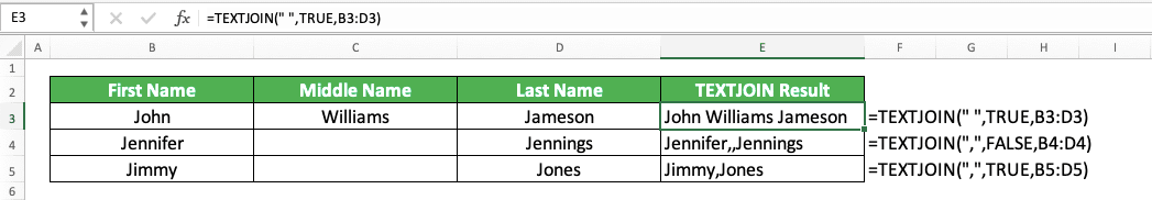
In the example, we use three different cases of TEXTJOIN to combine our names. In the first row, we use TEXTJOIN to combine the names normally using spaces as our separators ( “ “ ). As there isn’t any empty cell in the cell range that we input to TEXTJOIN, using TRUE/FALSE input doesn’t matter.

However, when we look at the second row, there is an empty cell in the middle name column. As we use FALSE in our TEXTJOIN there, the TEXTJOIN involves the empty cell in its combination process.

As a result, we get our text with empty data in between the first name and the last name. TEXTJOIN also gives a comma separator for the empty data in its result.

For the third row, it is almost the same as the second row but we use TRUE for the TEXTJOIN input. Because of that, TEXTJOIN ignores its cell range’s empty cell and only combines the cells with data. As a result, we get the first name and last name combined, separated by a comma symbol!

CONCAT with New Lines as Separators: TEXTJOIN & CHAR(10)

What if we want to use a new line as the separator in the text of our combined data? Is there a way to do this easily in excel?

Again, you shouldn’t use CONCAT, especially if you want to combine data in a cell range and it is quite large. You need to use TEXTJOIN instead with the help of the CHAR formula too (since we cannot type a new line as a separator directly to TEXTJOIN).

CHAR in excel can help you to get a character depending on the character code you input into it. As the new line character code is 10, that means you should input CHAR(10) to your TEXTJOIN. Input it as the TEXTJOIN’s separator input, of course.

Moreover, you must remember to turn on the wrap text setting in the cell where you write your TEXTJOIN CHAR. If you don’t, then you won’t see the new lines in your result.

To illustrate, here is the general writing form of TEXTJOIN and CHAR combination for the purpose.



And here is its implementation example in excel.



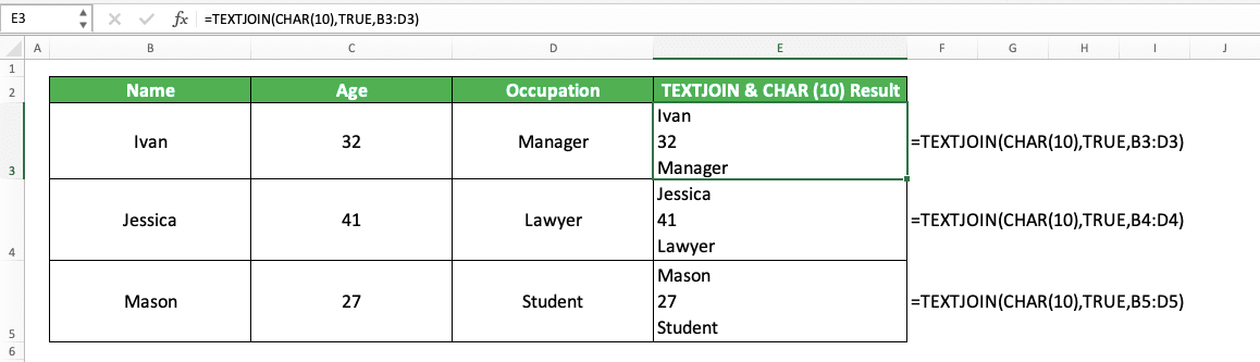
In the example, we can see that our TEXTJOIN results have new lines for each data it combines. That is because we input CHAR(10) as the separator input of our TEXTJOIN!

Besides the CHAR(10) as the input, we write the rest of our TEXTJOIN normally. As a result, we get the results that we want for our text!

Exercise

After learning how to use CONCAT in excel, now is the time to do some exercise to practice your understanding!

Download the exercise file and do all the instructions. Download the answer key file to check your answers or if you need a clue on how to run the instructions!

Link to the exercise file:
Download here

Questions

1. Unify all the numbers in the A and B columns into one text!
2. Unify all the numbers in the fourth, fifth, and ninth rows into one text!
3. Unify all the numbers from A3 to B5, D4, and C9 to E11 into one text!

Link to the answer key file:
Download here

Additional Note

• Whatever type of data that you combine with CONCAT (number, text, or other types of data), it will always produce a text
• If you input a cell range, then CONCAT will combine data from the top-left cell to the bottom right
• If you use dates as its input, then CONCAT will use the serial number of the date for its combination process

Related tutorials you should learn: