How to Use the MMULT Formula in Excel: Functions, Examples, and Writing Steps
Home >> Excel Tutorials from Compute Expert >> Excel Formulas List >> How to Use the MMULT Formula in Excel: Functions, Examples, and Writing Steps


In this tutorial, you will learn how to use the MMULT formula in excel completely.
When working with numbers in excel, we might sometimes need to multiply the number matrices we have. If we know how to use MMULT, then we can do that multiplication process easily.
Want to know more about MMULT and master the way to use it properly in excel? Read this tutorial from Compute Expert until its last part!
Disclaimer: This post may contain affiliate links from which we earn commission from qualifying purchases/actions at no additional cost for you. Learn more
Want to work faster and easier in Excel? Install and use Excel add-ins! Read this article to know the best Excel add-ins to use according to us!
Table of Contents:
- What is the MMULT formula in excel?
- MMULT function in excel
- MMULT result
- Excel version from which we can start using MMULT
- The way to write it and its input
- Example of its usage and result
- Writing steps
- MMULT not working? Possible reasons and solutions
- Count rows that contain specific data: SUM MMULT TRANSPOSE COLUMN
- Exercise
- Additional note
What is the MMULT Formula in Excel?
MMULT is an excel function that helps us to multiply number matrices in excel. We usually have our number matrices in the form of cell ranges in excel.MMULT Function in Excel
We can use MMULT to get the multiplication result of number matrices in excel.MMULT Result
MMULT result is a number matrix (array) that comes from the multiplication result of the matrices you input into it.Excel Version from Which We Can Start Using MMULT
We can start using MMULT in excel since excel 2013.The Way to Write It and Its Input
Here is the general writing form of an MMULT formula in excel.
{ = MMULT ( number_matrix1 , number_matrix2 ) }
You need to input the number matrices you want to multiply to MMULT to use the function.
As the result of MMULT is an array, you need to use the array formula form for this function. That means, to get all its results, you need to highlight the right size of cell range when writing the formula.
The cell range must have the same number of rows as your first number matrix input. It must also have the same number of columns as your second number matrix input. Furthermore, you should also press Ctrl + Shift + Enter buttons after you write your MMULT formula (instead of just Enter like when you write most excel functions formula).
Moreover, the number of columns in the first matrix must equal the number of rows in the second matrix. If this is not the case, then MMULT will produce a #VALUE error (because that is the general requirement of a number matrices multiplication process).
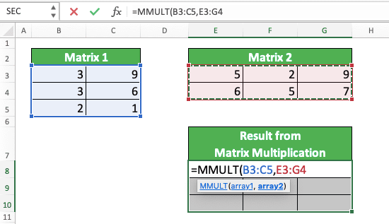
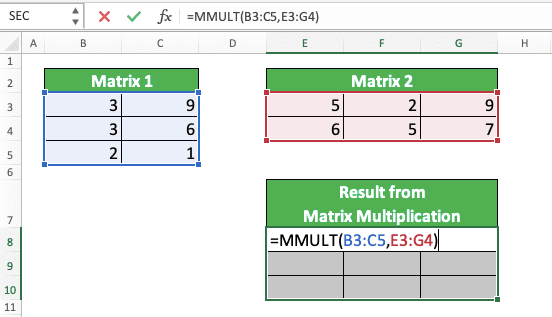
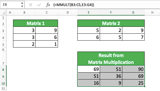
Example of Its Usage and Result
Here is an implementation example of MMULT in excel.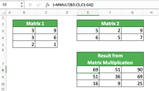
As you can see there, we can multiply our number matrices in excel by using MMULT. Just input the number matrices to the function and use the array formula form to do it.
Writing Steps
After we discussed the MMULT writing form, inputs, and implementation example, let’s discuss its writing steps. You can learn the detail of how we write MMULT correctly from the start to finish in excel here!-
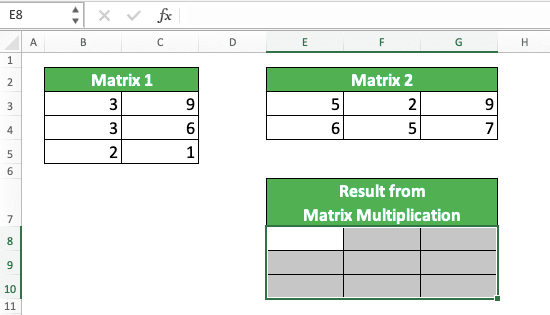
Highlight the cell range where you want to put the matrix multiplication result. The cell range must have the same number of rows as the first matrix you want to multiply. It must also have the same number of columns as the second matrix you want to multiply
-
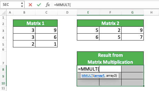
Type an equal sign ( = ), MMULT (can be with large letters and small letters), and an open bracket sign
-
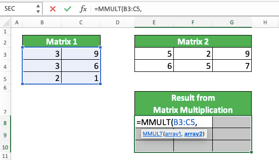
Input the first number matrix you want to multiply. Then, type a comma sign ( , )
-
Input the second number matrix you want to multiply
-
Type a close bracket sign
- Press Ctrl + Shift + Enter
-
Done!
MMULT Not Working? Possible Reasons and Solutions
Does your MMULT give a wrong result or even an error? There are many things that can cause that to happen. However, here are the three causes we think are the most possible and the solutions for each of them.- Reason: You don’t highlight the right size of cell range before you write your MMULT formula
Solution: Highlighting the wrong size of cell range to place your MMULT results will make you not get all its results. Make sure you highlight a cell range that has the right size before you write your MMULT formula. That means the cell range has your first matrix’s number of rows and your second matrix’s number of columns - Reason: You don’t press Ctrl + Shift + Enter after you write your MMULT formula
Solution: Pressing Enter instead of Ctrl + Shift + Enter will make your MMULT formula a normal formula, not an array formula. As the results of MMULT can be multiple, you should press Ctrl + Shift + Enter to ensure you get all its results - Reason: The number of columns in your first matrix isn’t the same as the number of rows in your second matrix
Solution: A Matrix multiplication requires the first matrix you multiply to have columns as many as the second matrix rows. Fix the columns and/or the rows of the matrices you input into MMULT if that isn’t the case
Check all these three things if you encounter a problem when you try to get the right results from your MMULT!
Count Rows that Contain Specific Data: SUM MMULT TRANSPOSE COLUMN
Need to count the number of rows in your cell range in excel that contains specific data? You can also use MMULT to do the counting process for you, with the help of SUM, TRANSPOSE, and COLUMN too.Here is the general writing form of those functions combination for the purpose in excel.
{ = SUM ( — ( MMULT ( — ( cell_range = specific_data ) , TRANSPOSE ( COLUMN ( cell_range ) ) ) > 0 ) ) }
After you write this formula, don’t forget to press Ctrl + Shift + Enter as you need an array formula form for this.
Want to know the logic behind this formula writing? Take a look at its implementation example below.
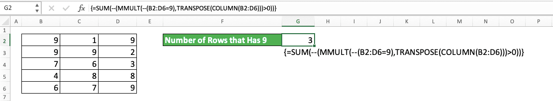
As you can see in the example, we can get the number of rows with 9 in our cell range (3). That is because we write our SUM, MMULT, TRANSPOSE, and COLUMN combination with the pattern we mentioned before.
How is the combination of the functions able to get the number of rows that contains specific data? First, let’s take a look at the first matrix input in our MMULT in the formula writing.
For that input, we input a logic condition where we compare our cell range with the specific data we want. The cell range is where we want to count the rows that contain the specific data.
From this logic condition, we will get an array of TRUE or FALSE. The TRUE or FALSE depends on whether each cell in the cell range contains the specific data we want or not. In the example, we get an array like this as a result of the logic condition.
{ TRUE , FALSE , TRUE ; TRUE , TRUE , FALSE ; FALSE , FALSE , FALSE ; FALSE , FALSE , FALSE ; FALSE , FALSE , TRUE }
Notice that we have TRUE where we have 9 in our cell range. That is because 9 is what we compare our cell range within our logic condition input.
After that, we convert our TRUE/FALSE array into a 1/0 array. We do it by using the double minus symbol ( — ) we put before our logic condition input. From that, we get this as a replacement for our TRUE/FALSE array.
{ 1 , 0 , 1 ; 1 , 1 , 0 ; 0 , 0 , 0 ; 0 , 0 , 0 ; 0 , 0 , 1 }
For the second matrix input in our MMULT, we input our cell range into our COLUMN inside our TRANSPOSE.
COLUMN gives us the column numbers of our cell range. Thus, we get this array from it.
{ 2 , 3 , 4 }
Our TRANSPOSE makes this one row, three columns array into one column, three rows array like this.
{ 2 ; 3 ; 4 }
We need to use TRANSPOSE so we can multiply the COLUMN result with our 1/0 array by using MMULT.
We get this array from those two arrays multiplication.
{ 6 ; 5 ; 0 ; 0 ; 4 }
Notice that we only get numbers more than 0 in the rows that have specific data we want (9 in this example).
We compare this array we get from MMULT with “larger than 0” in our formula writing. Thus, we get a TRUE/FALSE array again like this.
{ TRUE ; TRUE ; FALSE ; FALSE ; TRUE }
We turn this TRUE/FALSE result with a double minus we write before the comparison with “larger than 0”. Thus, we get this from the conversion of the TRUE/FALSE array.
{ 1 ; 1 ; 0 ; 0 ; 1 }
Next, we just let SUM finishes the job by summing all the numbers in that final array. We get 3 as a result, the same as the number of rows that have 9 in the example cell range!
Exercise
After you have learned how to use MMULT in excel properly, let’s do an exercise. This is so you can practice the tutorial lessons better.Download the exercise file and answer the questions. Download the answer key file if you have done the exercise and want to check your answers.
Link to the exercise file:
Download here
Instructions
- What is the multiplication result of matrix 1 and matrix 2? Give your answer by using the gray-colored cell as the most top left cell in your results cell range!
- What is the multiplication result of matrix 2 and matrix 1? Give your answer by using the gray-colored cell as the most top left cell in your results cell range!
- How many rows in matrix 2 have 2 in them? Combine SUM, MMULT, TRANSPOSE, and COLUMN to give your answer!
Link to the answer key file:
Download here
Additional Note
MMULT will produce a #VALUE error if you have anything other than numeric data in your matrix inputs (e.g. empty cells, texts, logic values, etc).Related tutorials you should read too: