How to Find a Name in Excel Sheet
Home >> Excel Tutorials from Compute Expert >> Excel Tips and Trick >> How to Find a Name in Excel Sheet
In this tutorial, you will learn completely how to find a name in an excel sheet.
Name is data we often save and process in excel. Sometimes, it can be difficult to find the name data we need for our data processing and analysis. Don’t worry, though. Because after learning this tutorial, you will understand how to find a name in excel fast and easily!
Disclaimer: This post may contain affiliate links from which we earn commission from qualifying purchases/actions at no additional cost for you. Learn more
Want to work faster and easier in Excel? Install and use Excel add-ins! Read this article to know the best Excel add-ins to use according to us!
Table of Contents:
How to Find a Name in Excel 1: The Find Feature
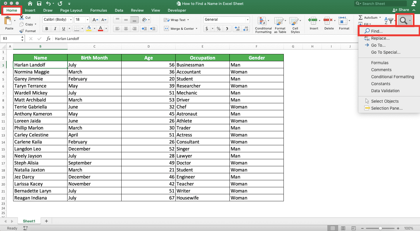
The first way to find a name in excel that we will discuss is by using the Find feature. This feature can help us find the location of various data we need in an excel sheet, not just names.If you want to use Find to find a name, then the way to do that is pretty easy. First, you must activate the dialog box of this feature. To do that, press Ctrl + F simultaneously or click the Find & Select button in the Home tab and choose Find…
To know the Find & Select button location and its Find… choice, look at the screenshot below.
After the dialog box shows up, type the name you want to find in its text box. Then, click the Find Next button.
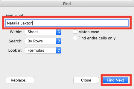
Excel will immediately move your cell cursor to the cell where the name you want to find is!

You have found the name you look for!
If you want to look at other places where the name is (if there is more), click the Find Next button again. If you want to find another name, then just fill that other name in the Find dialog box’s text box.
How to Find a Name in Excel 2: Filter
What if we have a table with many names and we want to display just one name in the table? That one name shows up a couple of times in the table and we want to show them simultaneously.Can we do that? Of course we can, by using the Filter feature in excel!
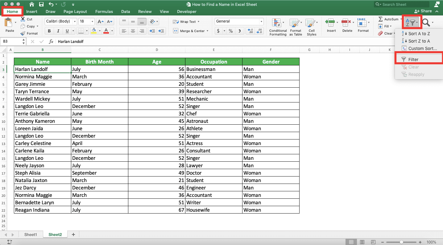
How to use this excel Filter feature for the purpose? First, you activate the Filter feature in your table by choosing Filter from the Sort & Filter dropdown in the Home tab. Do that when your cell cursor is in the cell range of your data table.
You can see the exact location of the Filter button below.
After you click Filter, there will be dropdown buttons in the headers of your data table like this.
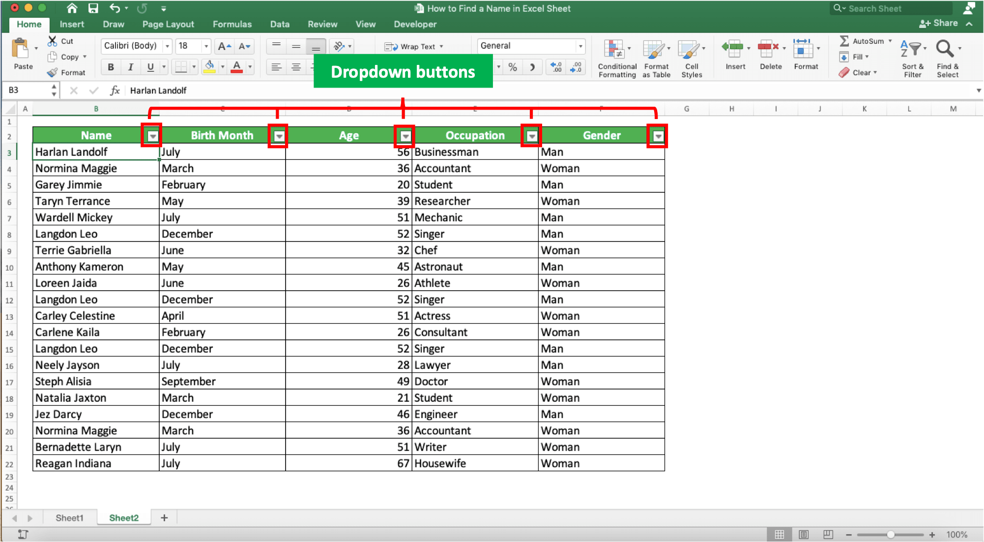
If you want to remove them after you find your name, then you can just click that Filter button again.
To begin finding the name, click the dropdown button in your name column header. After that, remove the checkmark in (Select All) so your data table doesn’t show any names. Then, click the checkbox of the name you want to find so all that name data are shown in your table.
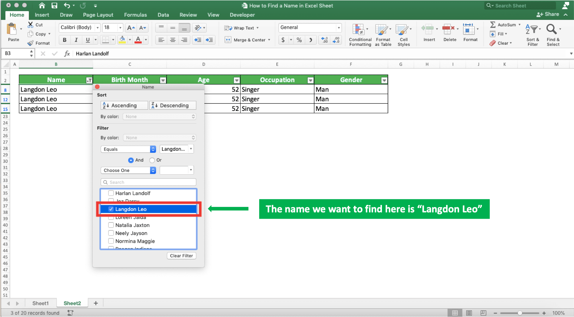
Close the filter dialog box by clicking the X mark at the top of the dialog box. You will get all instances from the name you want to find in your data table!

If you want to return your data table state, just click on the dropdown of the name column header again. Then, check the (Select All) checkbox by clicking on it.
How to Find the Same/Duplicate Names in Excel
When trying to find names in excel, we sometimes need to identify the same or duplicate names. Maybe, we need to delete those duplicates. Or, we need to know how many times the name is repeated for our data analysis purpose.If this is what you need, then you can use the IF and COUNTIF combination to help you identify the duplicates.
Generally, the way to write IF and COUNTIF for this purpose is as follows.
=IF(COUNTIF(name_column_cell_range, name)>1, name)
In the IF and COUNTIF writing, we input the COUNTIF in our IF. The COUNTIF is useful to check whether there are duplicates for a name. If there are, we use the name as a duplicate identifier. We don’t input a FALSE result in the IF because we don’t have a problem if IF produces FALSE for that.
We write this formula in a helper column that has the same size as our name column. The helper and name columns are better in line to make the name duplication identification process easier.
To make it clearer how to use the IF and COUNTIF, review its implementation in the following example. Let’s say we have data like this.
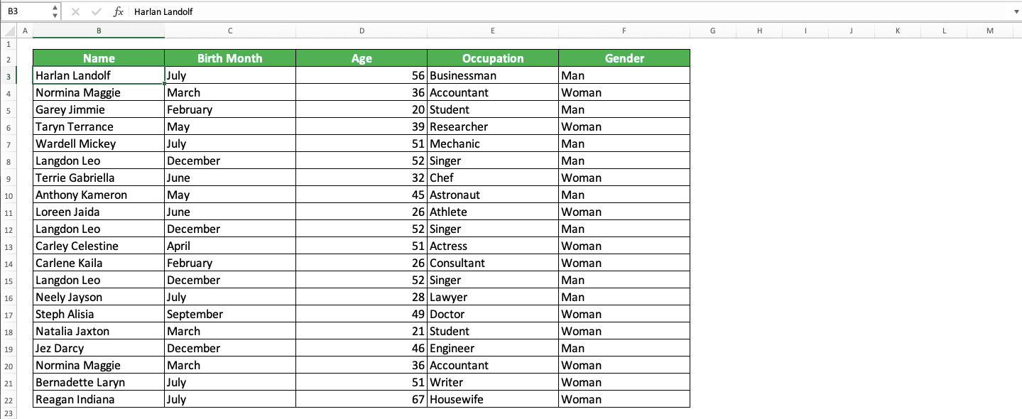
We want to know all the same/double/duplicate names in the data table. How to do it?
First, we prepare a helper column for this process where we will write our IF and COUNTIF combination. To make it simple, we can put it beside our name column like this.
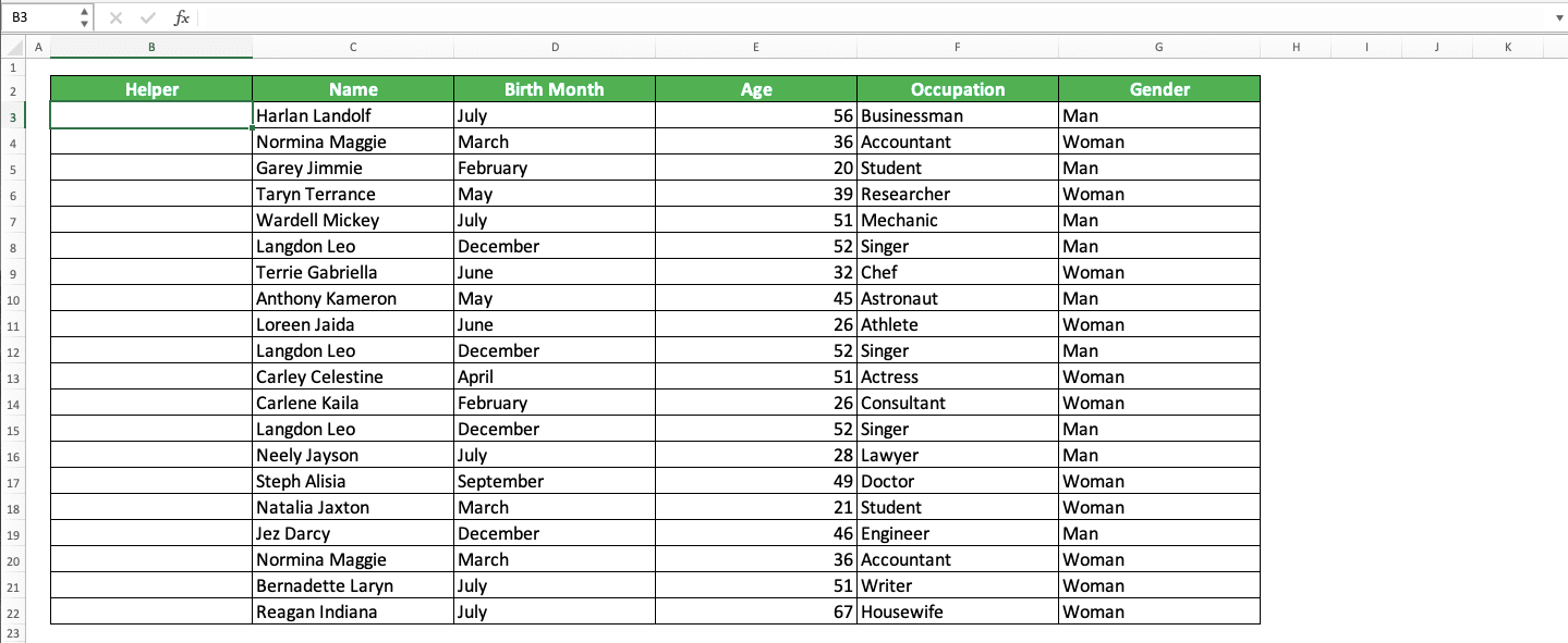
After getting the helper column ready, we write our IF and COUNTIF. The writing follows the form we discussed earlier.
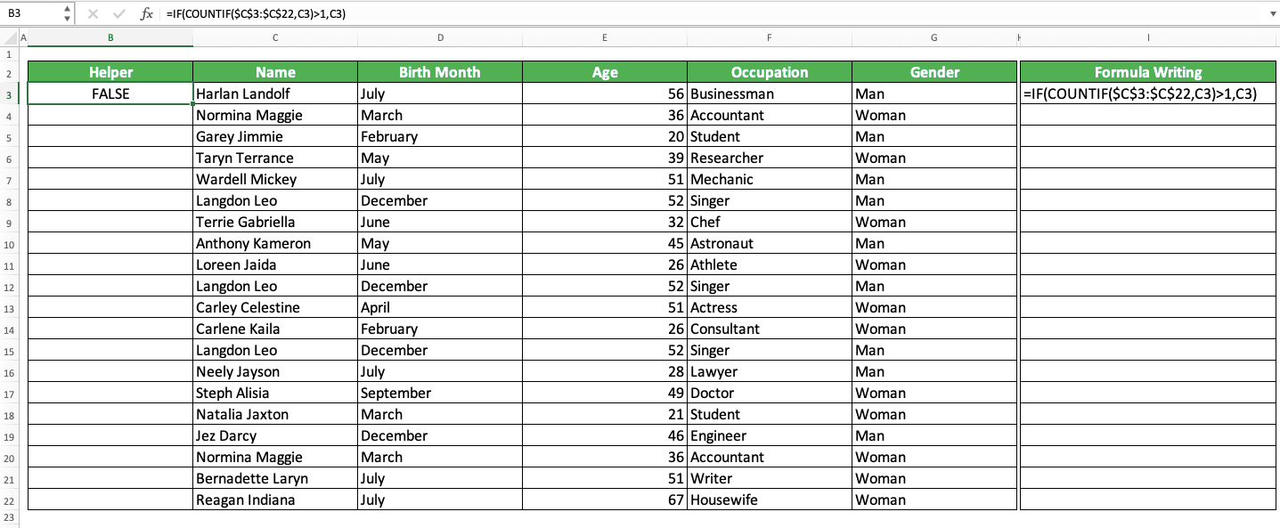
Look at the contents of the formula writing column so you can see the formula writing in the helper column clearer!
We can explain the process that the formula runs like this. COUNTIF there checks whether the name parallel to where the IF COUNTIF is written has duplicates or not.
We input the cell range where all the names are, with the count criterion is the parallel name. There are dollar symbols ($) in the cell range input because we want to copy the formula down later. We don’t want the cell range coordinate to move when we do the copy process.
If there are duplicates for the parallel name, then the COUNTIF result will be more than 1. Because of that, we input the logic condition that the COUNTIF result should be more than 1 in the IF. If TRUE, then there are duplicates and if FALSE, then there is no duplicate.
For the TRUE result input in the IF, we input the name we check. This is so we can know immediately the duplicated name and also as a unique identifier for the name.
For the FALSE result, we only need a mark that the name isn’t a duplicate. We don’t input anything there thus IF will give FALSE if there is no duplicate. This is as you can see in the “Harlan Landolf” name check in the example above.
After we write the IF COUNTIF, we copy the formula down so we can check the duplicate possibility of all names. As for the example, the copy results become like this.
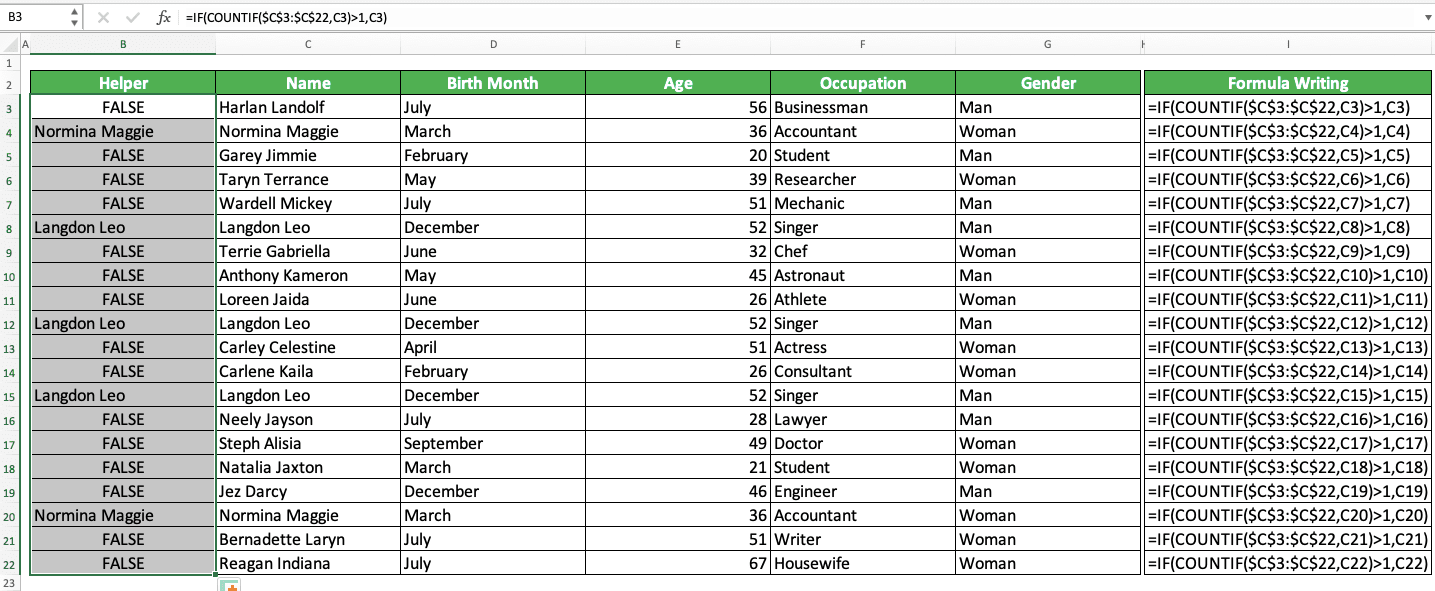
From there, we can see that the duplicated names there are Normina Maggie and Langdon Leo!
How to Find a Name in an Excel Sheet with a Lookup Reference Value: VLOOKUP/INDEX MATCH
Have a lookup reference you want to use to find a name in excel?You might have details about the name you want to find and you want to find it using those details. You can do that in excel by using the VLOOKUP and INDEX MATCH lookup formulas.
For VLOOKUP, here is how we write the formula generally.
=VLOOKUP(name_lookup_reference, cell_range, name_column_order, [TRUE/FALSE])
The TRUE/FALSE lookup mode input in the VLOOKUP depends on the reference lookup nature you want. If the reference is a number and we can lookup with the smaller nearest value to the reference, input TRUE. If we must find an exact match for the lookup reference, then input FALSE. If we don’t give any input here, then it will assume our input as TRUE.
If you use VLOOKUP, make sure the lookup reference is in the first column of your cell range.
For INDEX MATCH, the writing form is more or less like this.
=INDEX(cell_range, MATCH(name_lookup_reference, reference_lookup_column, [-1/0/1]), name_column_order)
Here, the assumption is we must find a row in the cell range to find the name data. For that, we put MATCH in the row position input of the INDEX.
In the MATCH, the lookup mode input can be -1/0/1. It depends on the lookup process you want to do with your reference. Here is a bit explanation for each input option for the MATCH’s lookup mode.
| Input | Lookup Nature | Explanation |
|---|---|---|
| -1 | Approximate | First, MATCH will try to find an exact match for your data. If it doesn’t find it, then it will look for smaller value data closest to the data you want. If you use this input, then your row/column cell range must be sorted in ascending order. |
| 0 | Match | First, MATCH will try to find an exact match for your data. If not found, then it will produce a #N/A error. |
| 1 | Approximate | First, MATCH will try to find an exact match for your data. If it doesn’t find it, then it will look for data with a larger value closest to the data you want. If you use this input, then your row/column cell range must be sorted in descending order. |
If you don’t input anything here, then it will assume your input as 1.
To make it clearer about this VLOOKUP/INDEX MATCH use, here is its implementation example to find a name in excel.
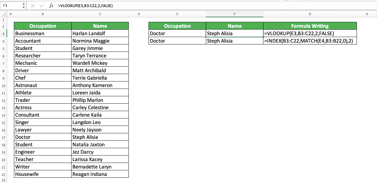
In the example, we can see how the VLOOKUP and INDEX MATCH produce the same results. Here, we use the “doctor” occupation as the lookup reference for the name data. Because the reference is a text, we use the exact lookup mode for the VLOOKUP and INDEX MATCH.
Write your formula correctly and give the right inputs to the formula you want to use. By doing that, you can get the name you want accurately and fast!
Exercise
After learning how to find a name in excel, let’s do an exercise. This is so you can understand more about how to implement the name lookup methods.Download the exercise file and do all the instructions. Download the answer key file too if you have done the exercise. Or probably when you are confused about how to run the instructions for the exercise!
Link to the exercise file:
Download here
Instructions
Do each instruction below in the appropriate sheet!- Sheet1: With the filter feature, try to find data entries with the name of “Rudy Kourtney”!
- Sheet2: With IF and COUNTIF, try to identify duplicate names in the data table! Mark the data row that has duplicate names with a yellow cell color!
- Sheet3: Try to find name data in the table on the left with the information in the table on the right! Find them using VLOOKUP/INDEX MATCH!
Link to the answer key file:
Download here
Additional Note
If you want to find again the name in your Find dialog box but you have closed it, press Shift + F4 (Command + G in Mac). By using the shortcut, you don’t need to open the dialog box again to find the name!Other tutorials you should learn:

LEN
Want to know how many characters you have in a name? Use LEN! Learn how to use the formula here!


