How to Sort in Excel
In this tutorial, you will learn how to sort in excel completely.
When working in excel, we sometimes need to sort data in order so we can analyze them much easier. Different types of data in excel may require different kinds of sorting method. With that in mind, we will discuss these sorting methods so you can sort what you need when working in excel.
Want to master ways to sort various data in excel? Read this tutorial until its last part!
Disclaimer: This post may contain affiliate links from which we earn commission from qualifying purchases/actions at no additional cost for you. Learn more
Want to work faster and easier in Excel? Install and use Excel add-ins! Read this article to know the best Excel add-ins to use according to us!
Table of Contents:
- How to sort alphabetically in excel
- How to sort numbers in excel in ascending/descending order
- How to sort names in excel
- How to sort by date in excel
- How to sort time in excel
- How to sort number IDs in excel
- How to sort highlighted cells in excel
- How to sort by color in excel
- How to sort duplicates in excel
- How to sort multi-level in excel
- How to sort subtotals in excel
- How to sort columns in excel
- How to sort a table in excel
- How to sort a pivot table
- How to sort charts in excel
- Exercise
- Additional note
How to Sort Alphabetically in Excel
We will start this tutorial by discussing the way to sort data alphabetically in excel.Sorting alphabetically is one of the basics when we talk about the process of sorting data anywhere. We can do this process in excel quite easily by following these steps.
-
Highlight the column cell range you want to sort alphabetically

-
Go to the Data tab and click the A to Z button or the Z to A button

-
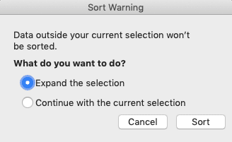
In the dialog box that shows up, there are two choices of sort process. Choose “Expand the selection”Choose “Continue with the current selection” if you want to only sort the column you highlight.
Click the Sort button after you choose
-
Done!

How to Sort Numbers in Excel in Ascending/Descending Order
Want to sort numbers in excel in ascending/descending order? The steps to do that are quite similar to how you sort your data alphabetically.Follow the previous steps to sort your data alphabetically to sort your numbers in excel. Highlight the cell range containing your numbers, go to the Data tab, and click one of the two sort buttons there. Excel changes the button names into “Sort Smallest to Largest” (ascending) and “Sort Largest to Smallest” (descending) when you want to sort numbers.
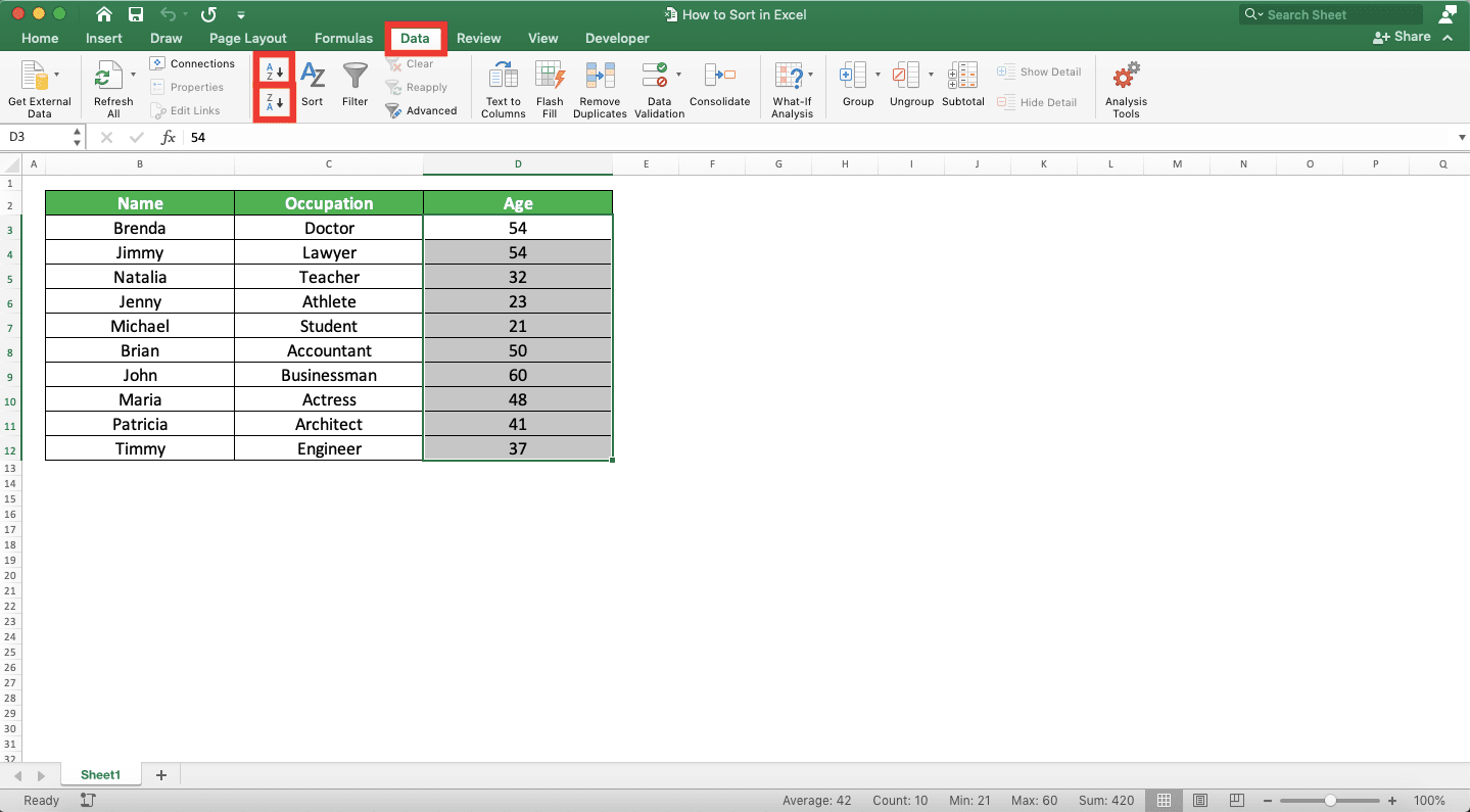
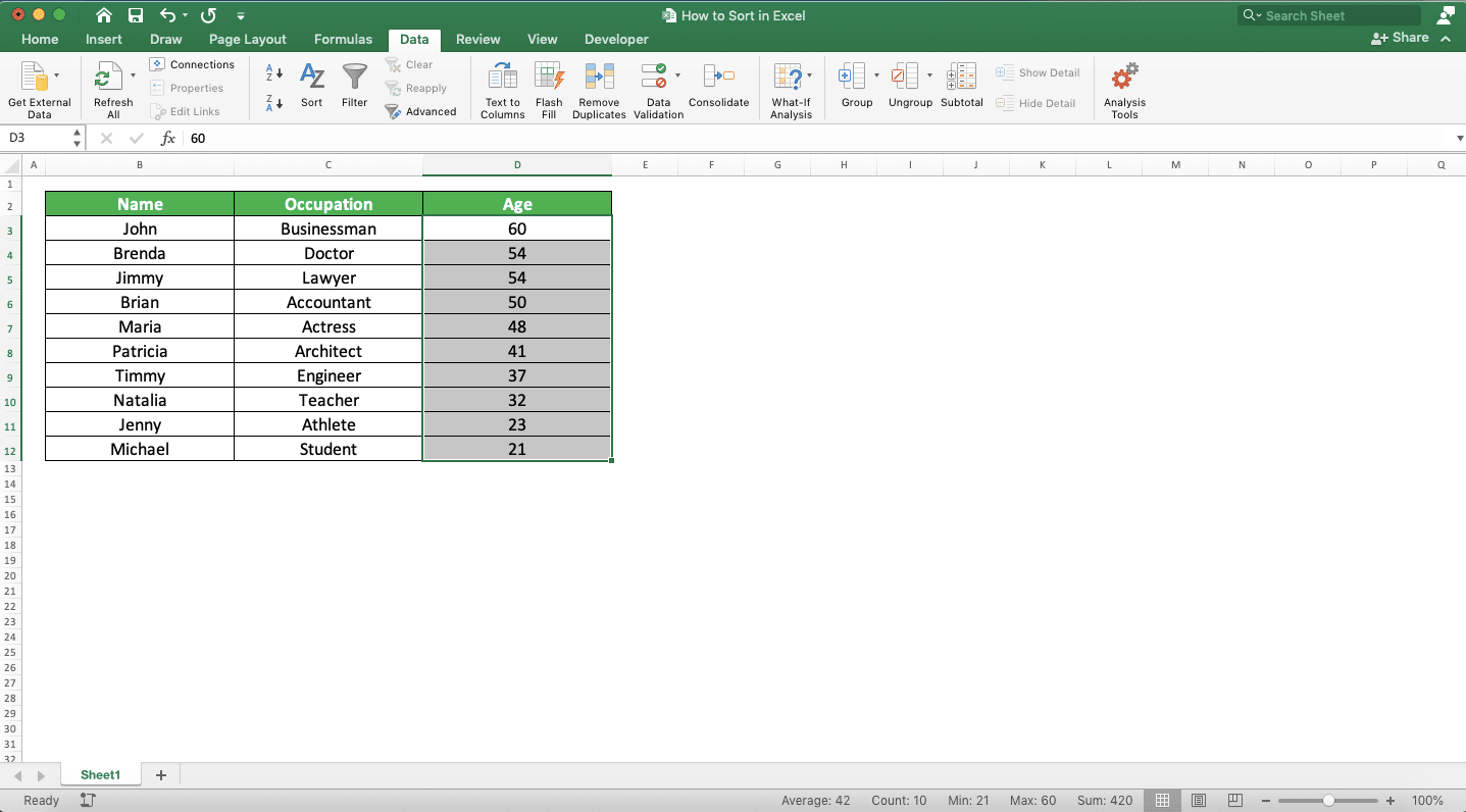
When you click the button, choose either “Expand the selection” or “Continue with the current selection”. Click the Sort button and you have sorted your numbers in the order you want!
How to Sort Names in Excel
Sorting names in excel are the same as sorting data alphabetically. You can either sort it from A to Z or Z to A.Just follow the previous steps to sort your data alphabetically in excel to sort your names. Doing that will make you able to organize your names in order!
How to Sort by Date in Excel
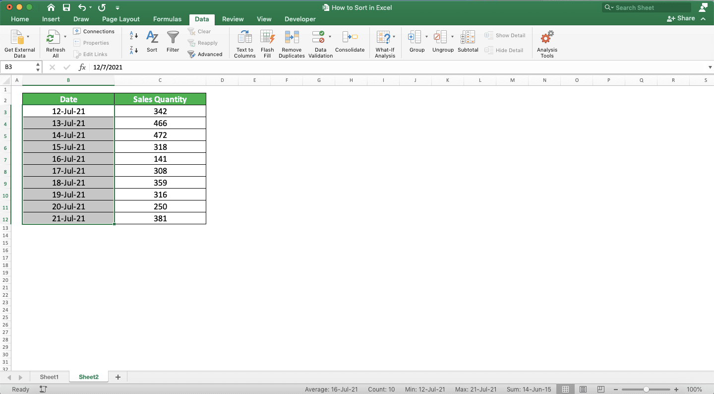
A date is a type of number data in excel. Therefore, the way to sort by date is quite similar to the way to sort numbers in excel.Highlight the cell range containing your dates, go to the Data tab, and click one of the two sort buttons there. You can either click the “Sort Oldest to Newest” or “Sort Newest to Oldest” button if you sort dates.

After that, choose either “Expand the selection” or “Continue with the current selection” in the dialog box that shows up. Click Sort and you have sorted your dates in the order you want!
How to Sort Time in Excel
Just as the date is, time is also a type of number data in excel. Therefore, you can also sort time in excel by using the method to sort numbers.Highlight the cell range containing the time, go to the Data tab, and click one of the two sort buttons there. You can click either the “Sort Smallest to Largest” or “Sort Largest to Smallest” button.
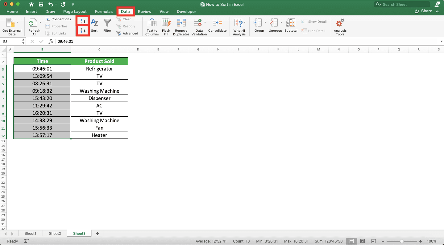
Choose “Expand the selection” or “Continue with the current selection” after that and then click Sort. You have sorted the time in your column in the order you want!

How to Sort Number IDs in Excel
To sort number IDs in a column, just use the numbers sorting method as number IDs are (obviously) numbers too.Highlight the number IDs column, go to the Data tab, and click one of the sort buttons there. You can either click the “Sort Smallest to Largest” or “Sort Largest to Smallest” button.
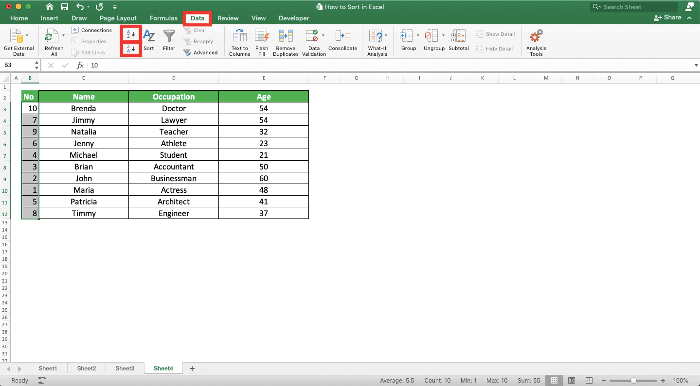
Choose “Expand the selection” or “Continue with the current selection” and click Sort. In the example, we choose “Continue with the current selection”.
Do all of those steps and you will immediately sort your number IDs in excel!

How to Sort Highlighted Cells in Excel
Need to sort data in some isolated, highlighted cells in excel? Just do it using the similar method we have discussed to sort data in excel.Keep highlighting the cells, go to the Data tab, and click one of the two sort buttons.
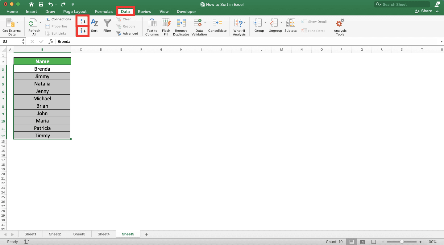
Do all that and you have sorted the data in your highlighted cells!

How to Sort by Color in Excel
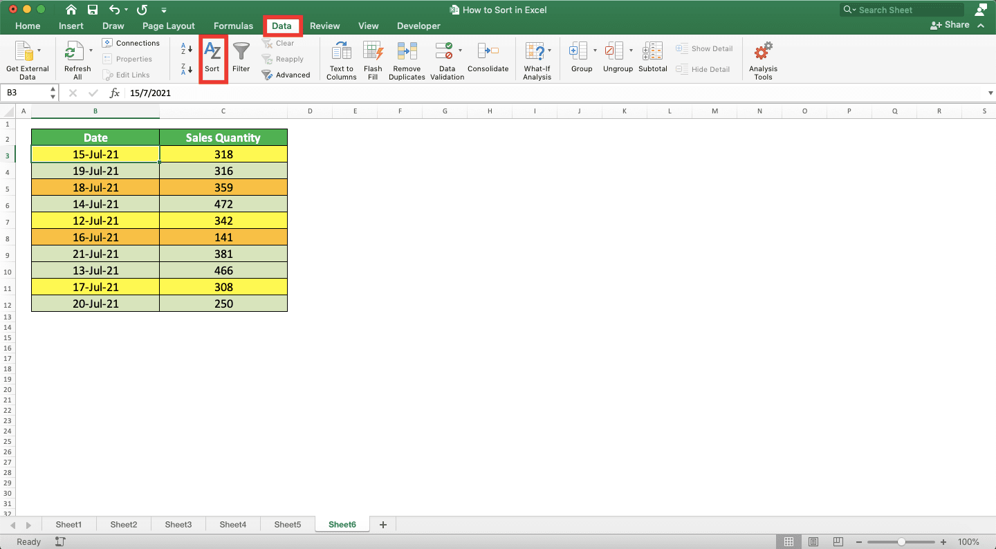
Have done some color coding in your data table and want to sort the table using the color as the basis? Follow the steps below to do the sorting process.-
Put your cell cursor in the cell range where you want to sort based on color

-
Go to the Data tab and click the Sort button there
-
In the dialog box that shows up, input the details of the color sorting process you want for your table. For each additional detail, you need to click the Insert button there.

In each detail, you need to input these:- The column which color you want to base your sorting process on in the “Column” dropdown
- The basis of the sorting process in the column in the “Sort on” dropdown. As you want to use color as the basis here, choose either “Cell Color” or “Font Color”
- The color you want to determine the sorting order of in the “Color/Icon” dropdown
- The order you want for the color you chose. On top or bottom
Give the details for all colors you want to base your sorting process on

-
Click OK. By doing these steps, you have sorted your data table by color!

How to Sort Duplicates in Excel
If you have duplicates in your data, you may want to sort them to the top to identify them much faster. To do this in excel, you can combine the usage of conditional formatting and the sorting process by color.We use conditional formatting to mark our duplicates first by color. To do that, highlight the cell range that contains data with duplicates you want to sort. Then, go to the Home tab, click the Conditional Formatting dropdown button, and choose Manage Rules….

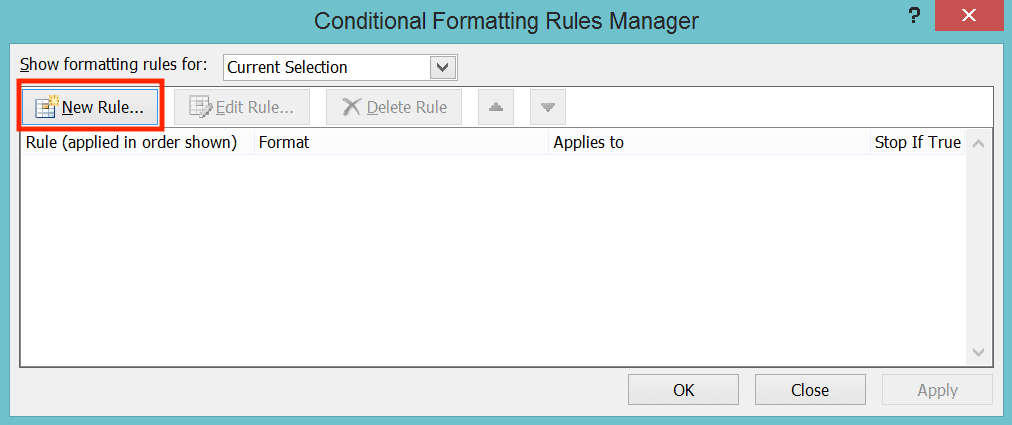
In the conditional formatting dialog box, click the New Rule… button.
In another dialog box that shows up, choose “Format only unique or duplicate values” in the Select a Rule Type box. Then, in the part below the box, make sure you select “Duplicate” in the dropdown.
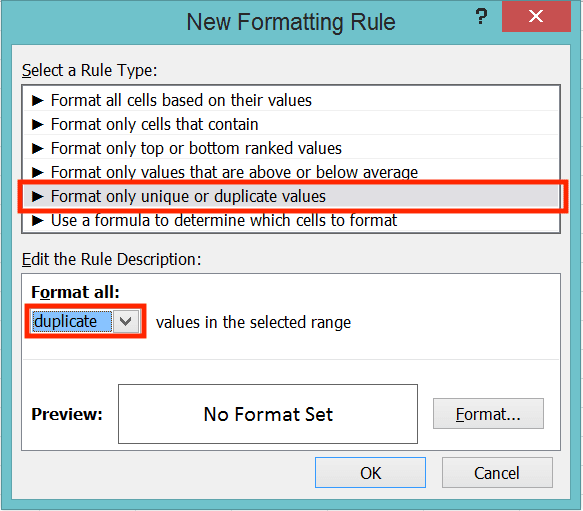
Next, click the Format… button.

As we want to color the duplicates, go to the Fill tab in the dialog box that shows up. Then, choose the color you want as the duplicates mark.
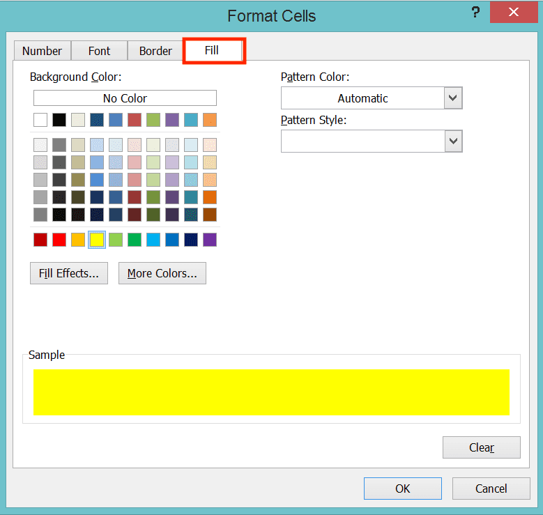
After you pick a color, click OK and then OK and then OK again. Now, the cells containing the duplicates in the cell range you highlight should have the color you picked.
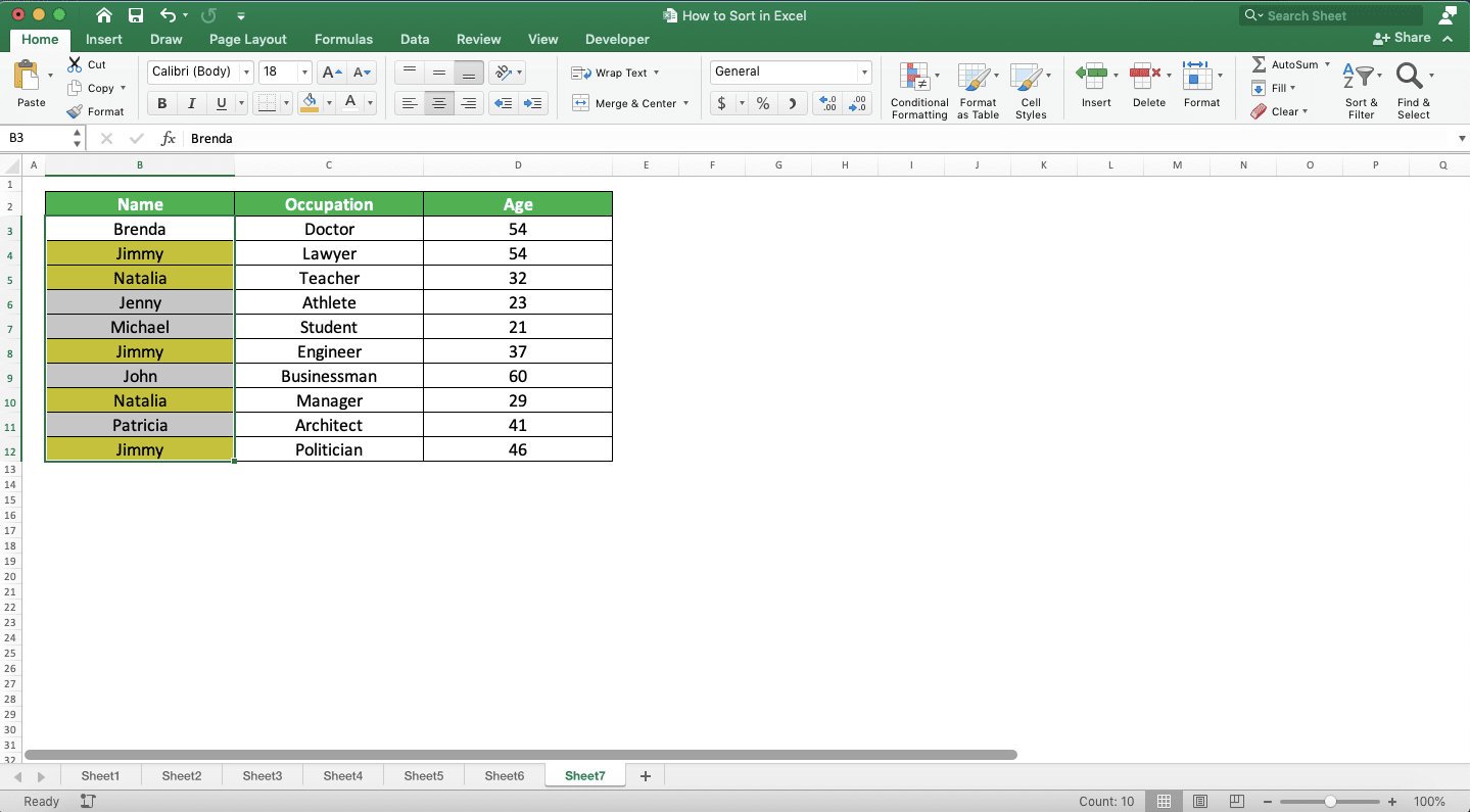
Next, we just need to sort our cell range based on the color of the duplicates. Put your cell cursor in the cell range with your data, go to the Data tab, and click the Sort button.
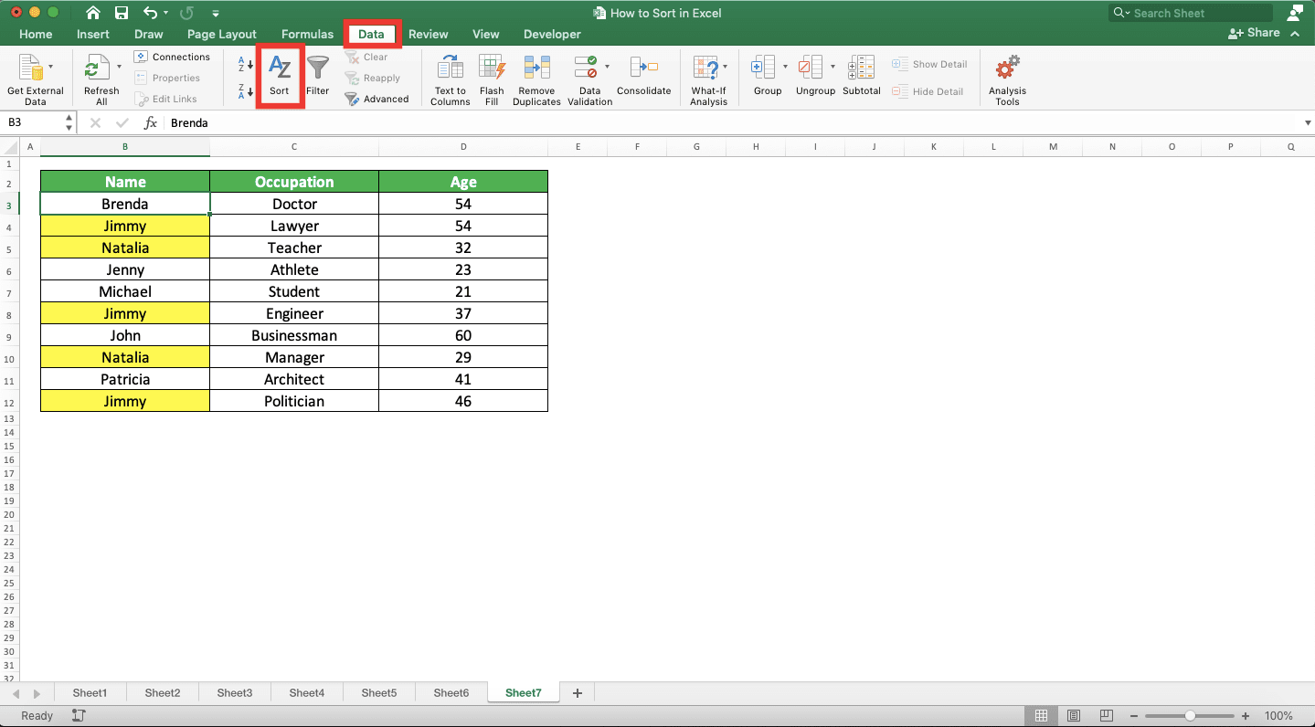
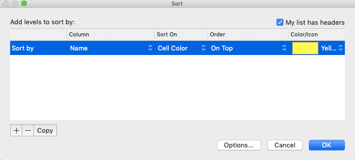
In the Sort dialog box, create a sorting detail that will make cells with the duplicate color go to the top. In the example, we choose the “Name” column, sort on “Cell Color”, “Yellow” color/icon, and “On Top” order.
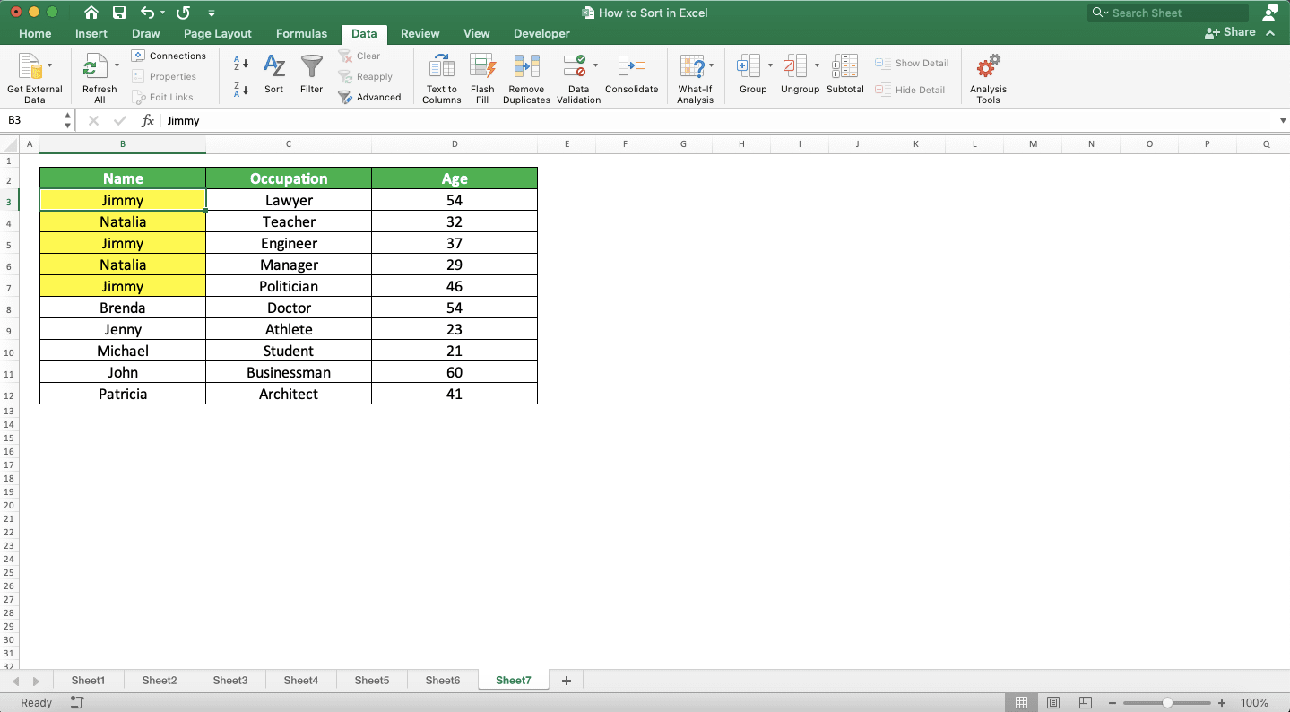
Click OK after you finish inputting the sorting detail. Now, your duplicates should be at the top of your cell range!
How to Sort Multi-Level in Excel
Need a multi-level sorting process for your data in excel?When you have this kind of needs, you might have multiple variables as the basis of your data table sorting process. There is a prioritization, of course, as we sort based on one variable first before we sort based on other variables.
We can do this sorting process by using the excel sort dialog box. Place your cell cursor in the data table where you want to do the multi-level sorting process. Then, go to the Data tab and click the Sort button there.

In the example, we want to sort based on the occupation first (A to Z) before we sort based on the name (Z to A). To do that, in the sort dialog box, we should create the details for both sorting processes.
The top detail in the dialog box is the one that excel will execute first. Thus, we create a sorting detail based on the occupation first here. We input the “Occupation” column, sort on “Values”, and “A to Z” order for the detail.
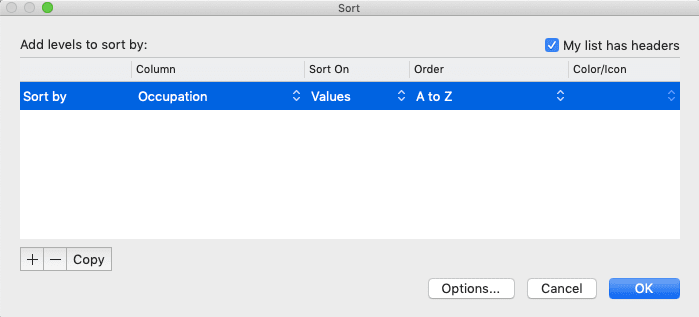
After we have done the first detail, we add another level to our sorting process based on names. To add that, we click the Insert button in the dialog box.

Clicking the button will add another line where we can input another sorting detail. Here, we input the “Name” column, sort on “Values”, and “Z to A” order.
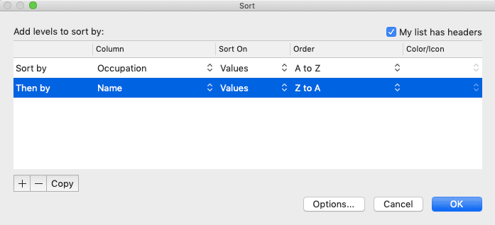
If you have other sorting levels you want to add, then keep clicking the Insert button and filling those lines. You can also move up/down the sorting levels and delete the ones you don’t need anymore in the dialog box.
Click OK after you have finished the sorting details input. Now, your data table should sort itself based on the sorting details you have inputted in the dialog box!

How to Sort Subtotals in Excel
If you use the subtotal feature in excel, then you can sort the subtotals of your numbers too if you want. The way to do the sorting process is quite simple.First thing you need to do obviously is to apply the subtotal feature to the numbers in your data table. If you haven’t done that, then place your cell cursor in the cell range where you want to get subtotals. Then, go to the Data tab and click the Subtotal button there.

Excel will show you the subtotal feature dialog box. Make sure the data variable you want to subtotal already has a checkmark in its check box there. Moreover, make sure the first dropdown places your subtotals in the right place and the second dropdown value is “Sum”.
In the example, we want the subtotals of sales quantity and we want to place them below each month. Therefore, our subtotal dialog box becomes like this.
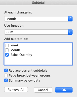
We click OK after that and excel will subtotal the numbers of the data variable we set in the dialog box!
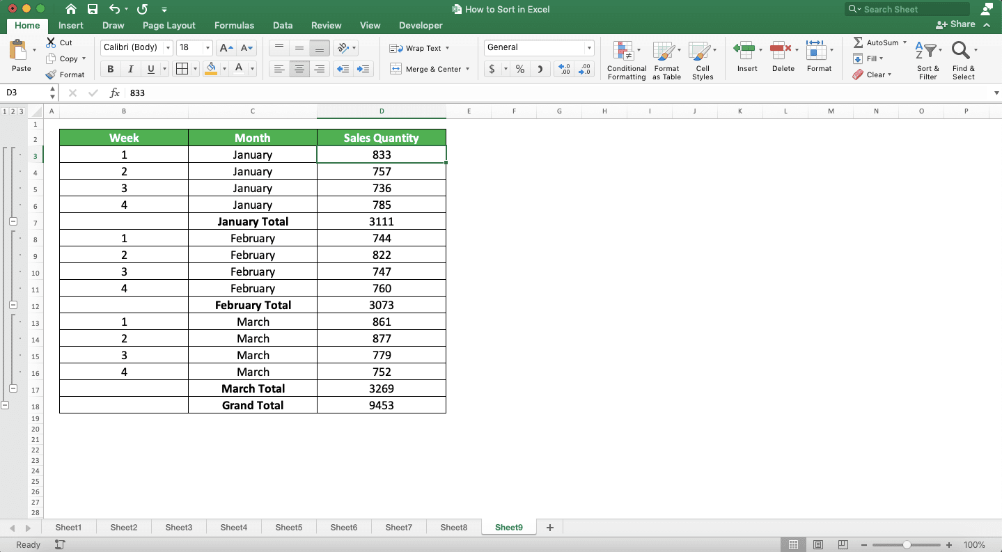
What comes with the subtotals is the data grouping settings that you can toggle at the left side of your worksheet. This grouping will become important if you want to sort your subtotals.
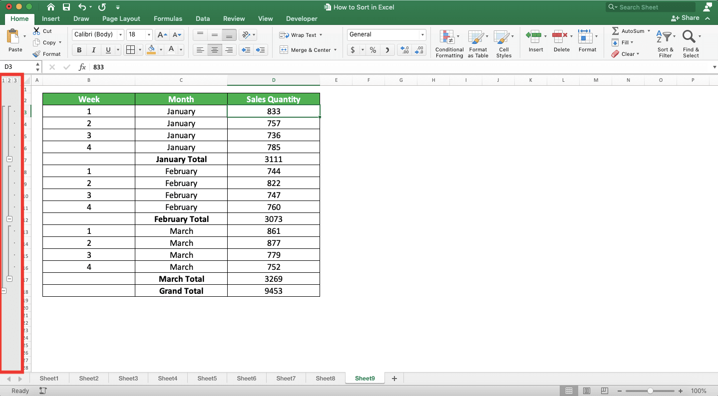
To start the subtotals sorting process, click all the minus symbols in line 2 on the left side.
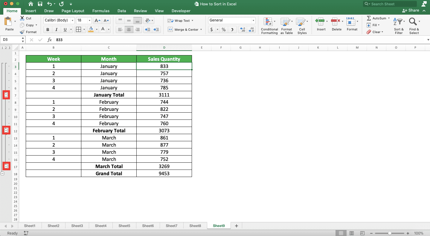
Doing that will make your data table only show the rows with the subtotal and total numbers.
Next, place your cell cursor in the column where your subtotals are. Then, go to the Data tab and click either the “Sort Smallest to Largest” or the “Sort Largest to Smallest” button. The button you should click obviously depends on the subtotals order you want in your sorting process.

Excel will immediately sort your subtotals based on the order you want! In the example here, we sort the subtotals from largest to smallest.
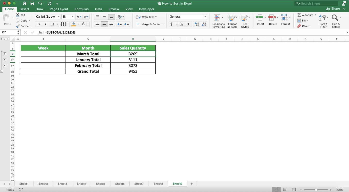
If you uncollapse your data again (by clicking the plus symbols on the left side), you will see that excel only sort your subtotals, not your numbers.

This is great if what you want is to only know the order of your subtotals without breaking your data order!
How to Sort Columns in Excel
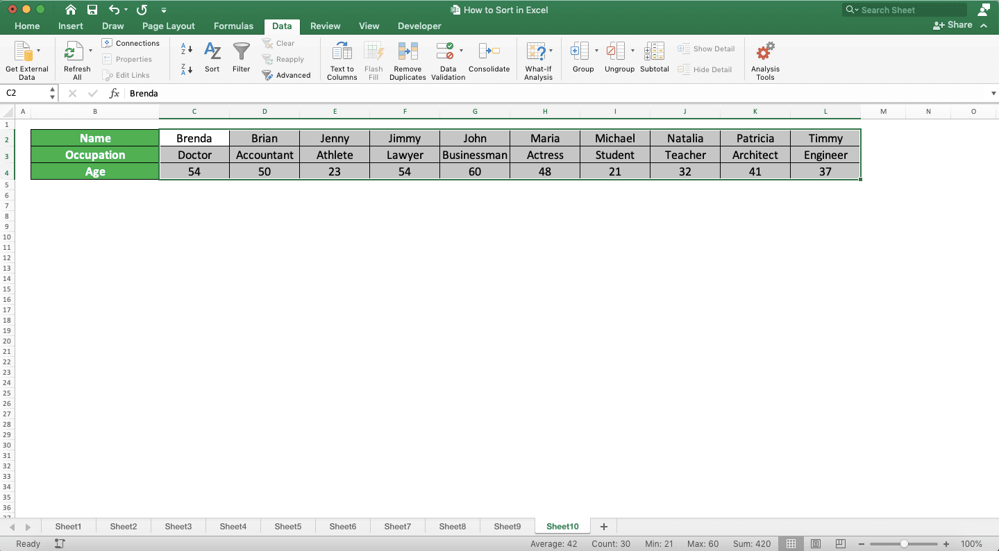
Your data in excel is in columns instead of rows and you want to sort it? Although uncommon, you can do that by changing few details to the usual sorting process.To start sorting your columns, highlight the columns which data you want to sort. Then, go to the Data tab and click the Sort button there.

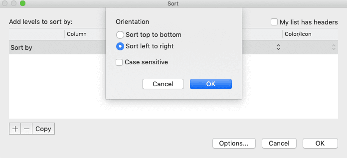
In the Sort dialog box, click the Options… button.

Choose the “Sort left to right” orientation and click OK.
Now, you can input the details of the sorting process for your columns! Choose the row which becomes the sorting basis (Row), what to sort there (Sort on), order (Order), and the color/icon (Color/Icon) to sort if any. For this example, we input Row 2 (Row), Values (Sort on), and A to Z (Order).
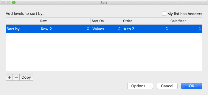
Click OK after you have inputted all the sorting details for your columns. Doing that will sort your columns according to your sorting detail inputs!
How to Sort a Table in Excel
As an excel table already has its own sort feature, it is quite easy to sort the data in it.To start doing the table sorting, first make sure your headers already have their filter buttons. They are the buttons with the down arrow on the right side of your headers.

They usually show up right after you convert a cell range into a table. If they don’t, then you can show them by checking the “Filter Button” check box in the Table tab. Place your cell cursor inside your table so the Table tab shows up in your ribbon.

If the filter buttons are there, click the button on the column you want to base your sorting process on. Then, choose whether you want to sort the column data in ascending or descending order.
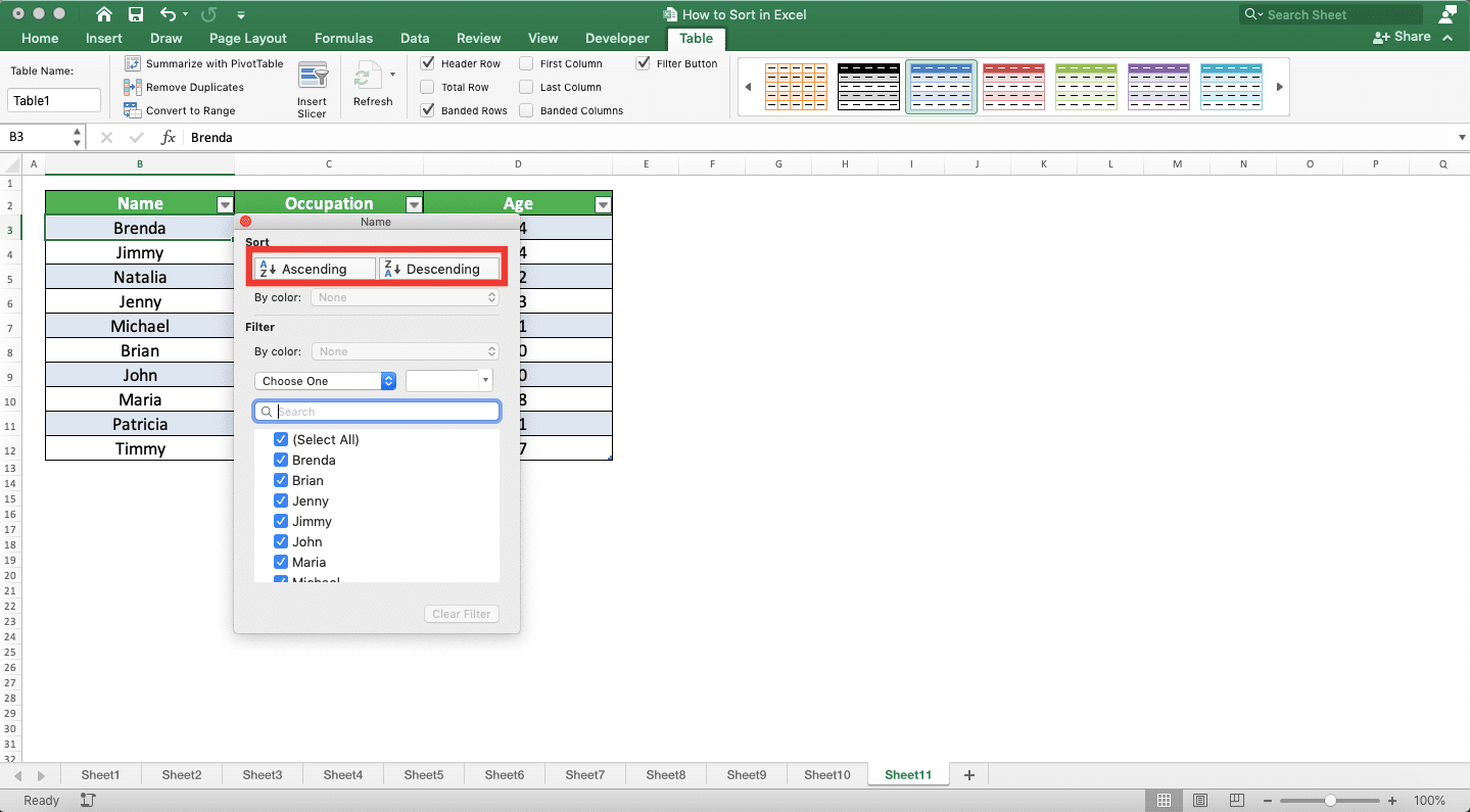
Doing that will make your table sort its data according to your preference!

How to Sort a Pivot Table
Want to sort the data you have in your pivot table? You can do it just like when you want to sort data in a standard data table in excel.Place your cell cursor in the column/row/value that you want to base your pivot table sorting process on. Then, go to the Data tab and click either the “Sort in Ascending Order” or “Sort in Descending Order” button (the names of the buttons depend on the type of data you want to base your sorting process on).
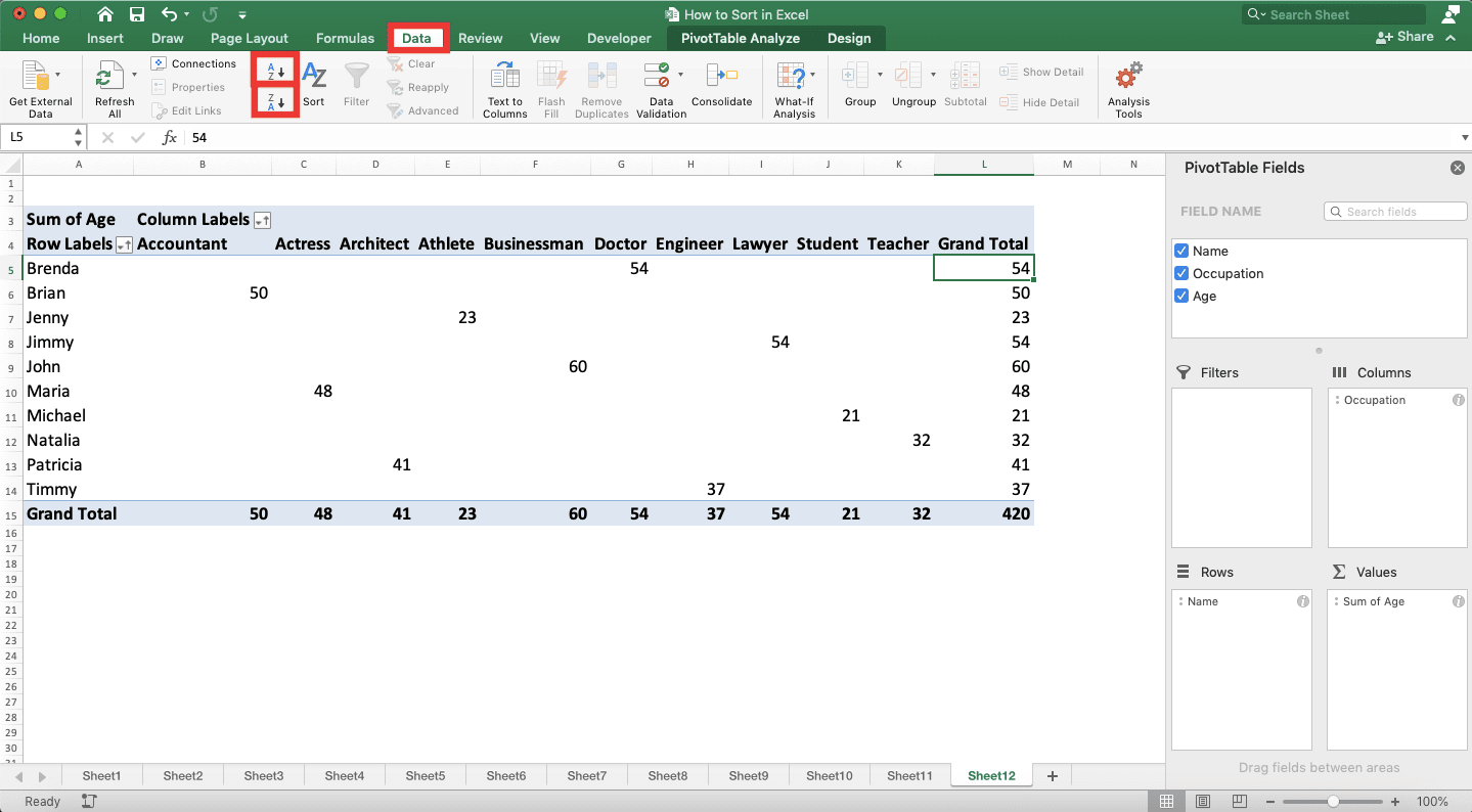
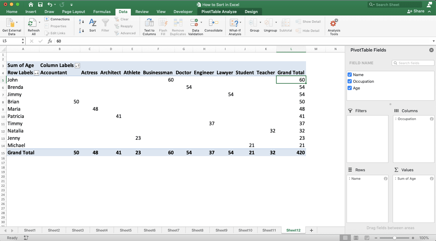
Done! You have sorted your pivot table based on the column/row/value you want!
How to Sort Charts in Excel
Need to sort your chart so it shows your data in an ascending/descending manner? You can do that by sorting its data source as the chart display should follow suit after that.You can sort the data source by using the standard steps to sort data in excel we have previously discussed. Place your cell cursor in the column you want to base your chart sorting process on. Then, go to the Data tab and click the “Sort in Ascending Order” or “Sort in Descending Order” button.
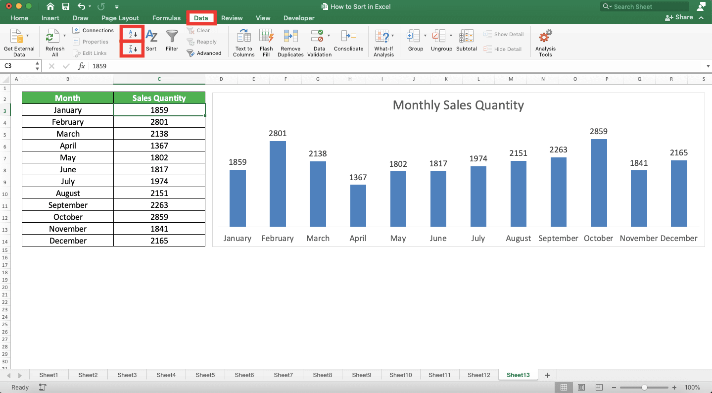
Do that and you have sorted your chart display!
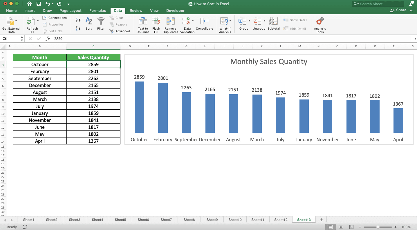
Exercise
After you have finished learning how to sort in excel from this tutorial, let’s do an exercise here. This is so you can understand what you have just learned more practically.Download the exercise file and answer all the questions. Download the answer key file if you have done the exercise and want to check your answers
Link to the exercise file:
Download here
Questions
Answer these questions in the appropriate gray-colored cells in the exercise file!- What is the date, product, and amount sold at the top if you sort the table based on the highest sales?
- What is the date, product, and amount sold at the bottom if you sort the table based on the newest sales?
- What is the fifth date, product, and amount sold if you sort the table with the following sorting details? Sort the green cells first to the top before you sort the data with red font colors
Link to the answer key file:
Download here
Additional Note
You can also sort by right-clicking the cell range you want to sort or by using the filter button. To activate the filter button, place your cell cursor in the data table you want to sort first. Then, go to the Home tab, click the Sort & Filter dropdown button, and choose Filter.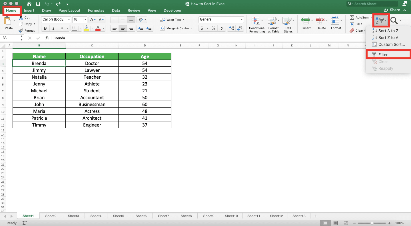
There will be down arrow buttons show up in your table headers. You can click the button in the header on which data you want to base your sorting process on. Then, choose sort in ascending order or in descending order.
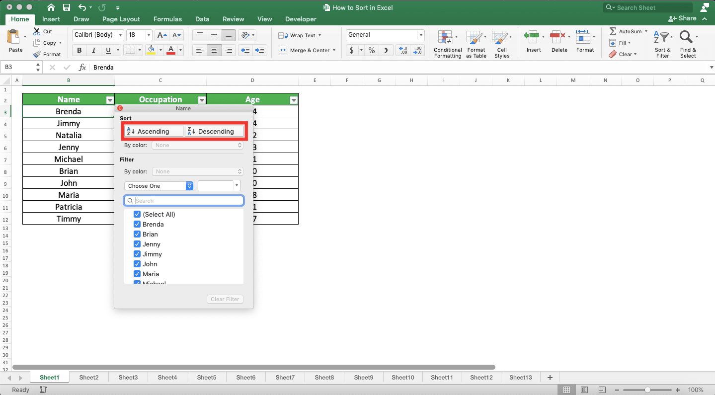
By doing that (or by choosing the relevant Sort command in the right-click menu), you have sorted the data in your table using the basis that you prefer!
Related tutorials you should learn too:


