Using IFERROR VLOOKUP Combination in Excel
Home >> Excel Tutorials from Compute Expert >> Excel Formulas List >> Using IFERROR VLOOKUP Combination in Excel


In this tutorial, you will learn how to combine IFERROR and VLOOKUP formulas in excel. This combination is sometimes needed to anticipate an error from the data lookup process done by VLOOKUP.
Disclaimer: This post may contain affiliate links from which we earn commission from qualifying purchases/actions at no additional cost for you. Learn more
Want to work faster and easier in Excel? Install and use Excel add-ins! Read this article to know the best Excel add-ins to use according to us!
Table of Contents:
- The usefulness of IFERROR VLOOKUP combination
- The result from IFERROR VLOOKUP combination
- The excel version from where this formula combination can be used
- A brief explanation for IFERROR and VLOOKUP separately
- The factors that can cause VLOOKUP to produce an error
- The writing method and input
- The example of usage and result
- The writing steps
- Nested IFERROR VLOOKUP
- The alternative for IFERROR VLOOKUP 1: IFNA VLOOKUP
- The alternative for IFERROR VLOOKUP 2: IF ISERROR/ISNA VLOOKUP
- Exercise
- Additional note
The Usefulness of IFERROR VLOOKUP Combination
IFERROR and VLOOKUP are combined so we can anticipate the error produced by VLOOKUP and substitute it with another value.VLOOKUP is a data lookup formula. One main reason why it can produce an error is it can’t find the data we look for. IFERROR helps us to ensure the error produced is replaced with other data that supports our data processing better.
The Result from IFERROR VLOOKUP Combination
The result of this combination is the normal result from VLOOKUP if the VLOOKUP doesn’t produce an error. However, if it produces an error, then the alternative value we give in our IFERROR becomes the result.The Excel Version from Where This Formula Combination Can Be Used
VLOOKUP can be used since excel 2003 while IFERROR can be used since excel 2007. Because of that, the IFERROR VLOOKUP combination can be used since excel 2007 (the earliest excel version where the two formulas are available to use)A Brief Explanation for IFERROR and VLOOKUP Separately
IFERROR is a formula that can be used to anticipate the error value of a process/data. Usually, it is used in a combination writing with another formula. One of its most often usage seems to be with this VLOOKUP formula.Briefly, IFERROR writing can be illustrated as follows:
=IFERROR(value, value_if_error)
Note:
- value = data or process that wants to be evaluated whether it has an error value or not
- value_if_error = the alternative value produced by IFERROR if it is true the data or process is an error
The use of IFERROR is not complicated because it is clear what should be given in its two parts of inputs. If you want to learn more about IFERROR, then take a look at this Compute Expert tutorial which discusses it.
Another part of the combination is the VLOOKUP formula. VLOOKUP is a vertical data lookup function provided by excel. About this formula writing itself, briefly, it can be illustrated as follows:
=VLOOKUP(lookup_value, table_array, col_index_num, range_lookup)
Note:
- lookup_value = your data lookup reference value to be searched in the first column of your reference table
- table_array = your reference table cell range
- col_index_num = the left-to-right order of the reference table column where the result of this formula will be taken
- range_lookup = optional. Determines whether your reference value lookup process will be exact or approximate. Input TRUE for approximate and FALSE for exact
If you want to learn further about this VLOOKUP formula, please visit the Compute Expert tutorial which discusses it!
The Factors that Can Cause VLOOKUP to Produce an Error
Here are the factors which usually cause VLOOKUP to produce an error and need a combination with IFERROR.- The lookup reference value cannot be found
- The use of TRUE as the input for the nature of the lookup process. In the case of an error, the first column of the inputted cell range probably hasn’t been sorted in ascending order
- The wrong inputs for the cell range and/or the column order where it should take the result
Because its function is to lookup data, then the error type often produced by VLOOKUP is #N/A (Not Available). The #N/A error is the excel way to tell the data we want as a result isn’t there/isn’t available.
The Writing Method and Input
Generally, the IFERROR and VLOOKUP combination writing can be illustrated as follows:
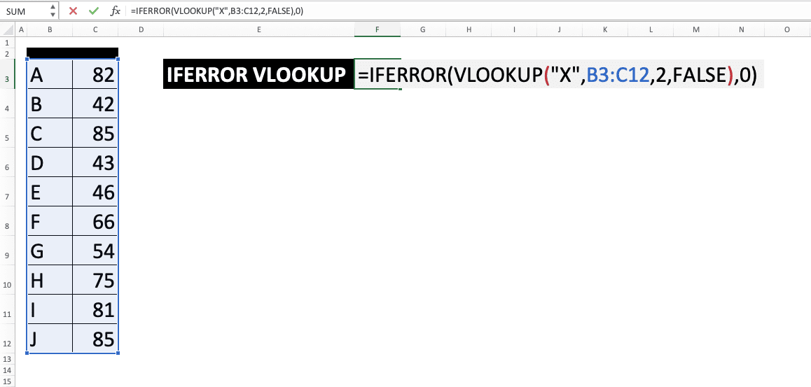
=IFERROR(VLOOKUP(lookup_value, table_array, col_index_num, range_lookup), value_if_error)
The inputs of this writing is the same as the inputs of the IFERROR and VLOOKUP formulas separately (explained in the previous part of this tutorial). The alternative values usually given for the VLOOKUP error are sentences like “Not Found” or just empty data (“”).
The Example of Usage and Result
The following will give and explain the usage and result example of the IFERROR VLOOKUP combination in excel.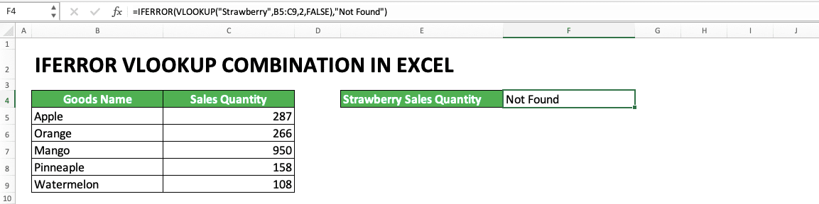
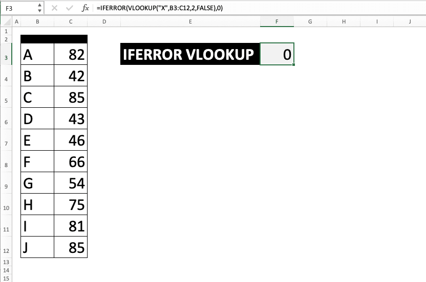
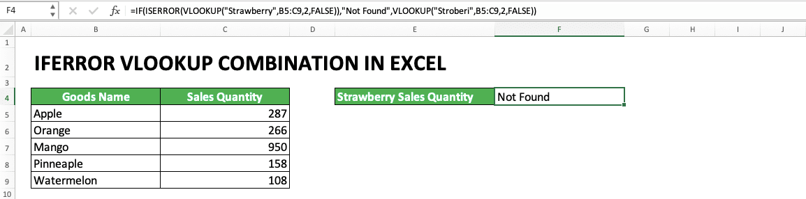
In the example, we can see a case where VLOOKUP produces an error because it doesn’t find the data. We can see the IFERROR VLOOKUP writing in the formula bar to give the “Not Found” text when the error happens.
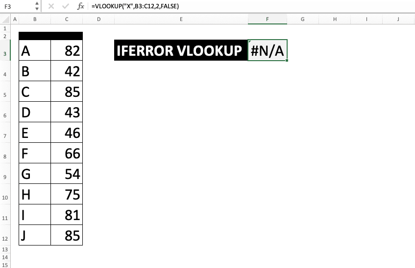
If we don’t use IFERROR in the VLOOKUP writing, then the result becomes a #N/A error. If we want to use the VLOOKUP result for further data processing, this error can cause other errors. Because of that, the VLOOKUP and IFERROR combination can be important to be implemented as a part of our data processing.
Want to input and process data in excel faster? Try using the XLTools Add-Ins! Use our discount coupon code “7C2L8B31AZ” to get a 10% discount when purchasing the Add-Ins license!
The Writing Steps
After discussing the example, now we will give the detailed step-by-step writing of the IFERROR VLOOKUP formula. Each step will be explained with a screenshot to ease your understanding.-
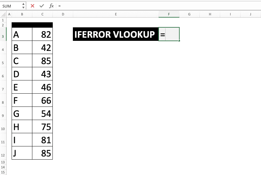
Type an equal sign ( = ) in the cell where you want to put the formulas combination result
-
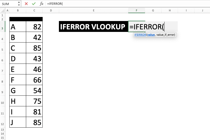
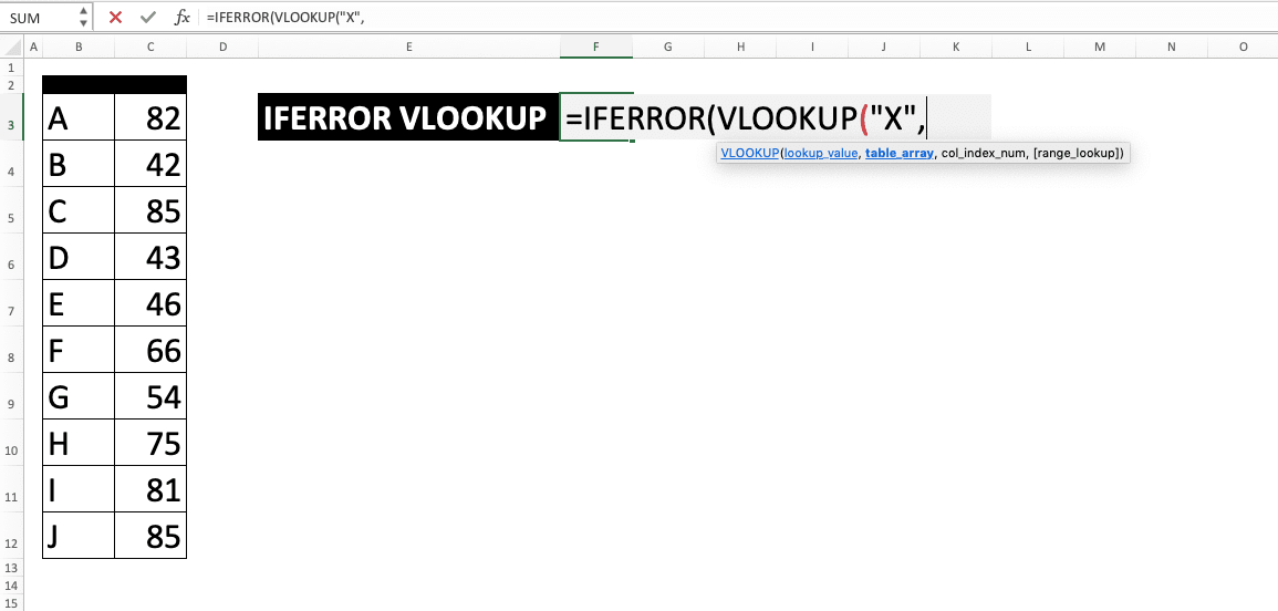
Type IFERROR (can be with large and small letters) and an open bracket sign after =
-
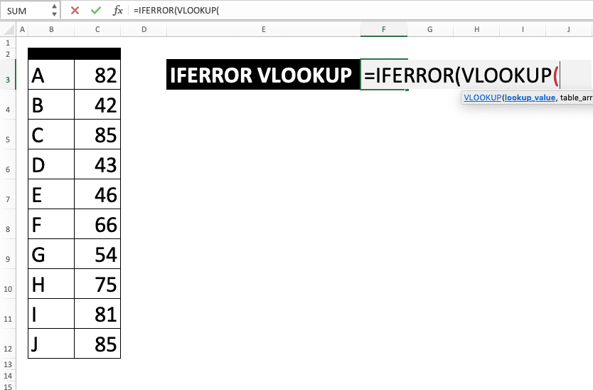
Type VLOOKUP (can be with large and small letters) and an open bracket sign
-
Input the lookup reference valu or the cell coordinate where this value is. Then, type a comma sign ( , )
-
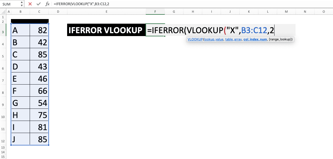
Input the whole cell range as a location to look for your data and type a comma signon the cell range where the search process will be done then type comma sign. Later, your lookup reference value will be searched in the first column of this cell range

-
Input the left-to-right order where the VLOOKUP result wants to be found in the cell range. The data taken for the result will be determined by the row position where your reference value is found. If there are more than one rows where your reference value is found, then the top row will be taken
-
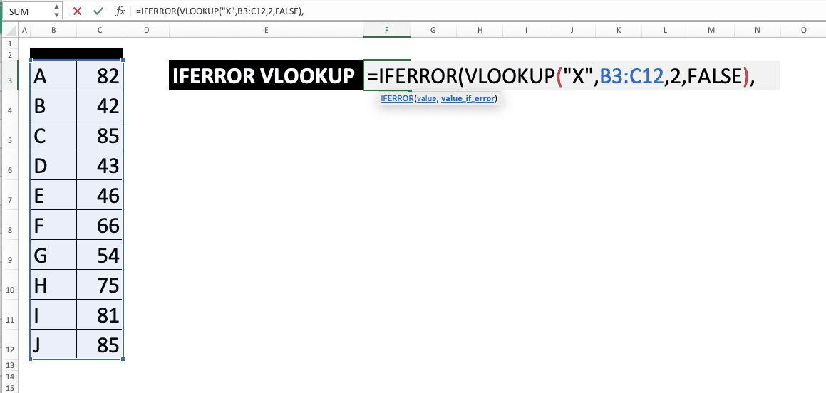
Optional: Optional: To determine whether the lookup value must be found exactly or approximately, input a comma sign and type TRUE/FALSE (not case-sensitive). TRUE for approximate and FALSE for exact.
Approximate means if there is no exact match for your reference value, VLOOKUP will take find smaller closest data to it. If you input TRUE here, then make sure your cell range first column has been sorted in ascending order. If it isn’t sorted, then VLOOKUP can give a wrong result!
If you don’t give input in this part, then the input will be considered as TRUE

-
Type a close bracket sign and a comma sign
-
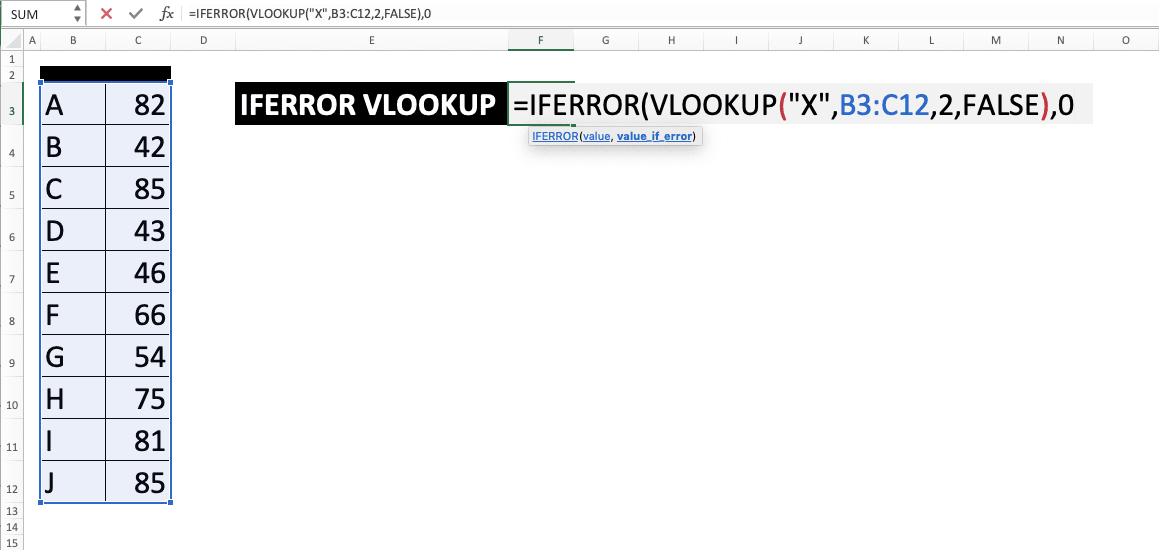
Type an error alternative value or the cell coordinate where the value is. This is a value that will be produced if your VLOOKUP produces an error
-
Type a close bracket sign
- Press Enter
-
Done!
The result with IFERROR
The result without IFERROR
Nested IFERROR VLOOKUP
Want to anticipate your error by looking for the data at another reference table? Then, you can use nested IFERROR VLOOKUP. By using it, you can look for your data in more than one place as you need.The method is by inputting another combination of IFERROR VLOOKUP in the error alternative value input part of your IFERROR. Do this repeatedly until all your data lookup places have been inputted.
A clearer understanding of this writing can be gotten by looking at the screenshot below.
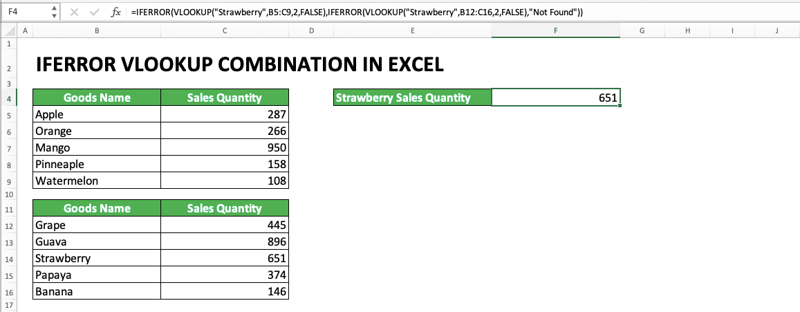
In the screenshot, you can see when VLOOKUP can’t find strawberry in the first table, it looks up the second table. There, it finds the strawberry sales quantity (651).
Make sure your nested IFERROR VLOOKUP writing is correct so you don’t produce the wrong result from your data lookup process!
The IFERROR VLOOKUP Alternative 1: IFNA VLOOKUP
Besides using IFERROR, you can also anticipate the #N/A error specifically that shows up from VLOOKUP with IFNA. The way to combine IFNA and VLOOKUP is similar to the IFERROR VLOOKUP combination, which has been explained earlier.
You need to remember, though, that IFNA will only anticipate a #N/A error and won’t anticipate other error types. If you need to anticipate all errors probably produced by the VLOOKUP, then use the IFERROR VLOOKUP combination.
The IFERROR VLOOKUP Alternative 2: IF ISERROR/ISNA VLOOKUP
If you still use the 2003 version of excel, then IFERROR or IFNA is still not available in your excel. Because of that, you can use the combination of the IF, ISERROR/ISNA, and VLOOKUP formulas instead.
This combination can also be used when you want to produce other data besides your lookup result. The data will be produced if your VLOOKUP can find the data you look for.
This alternative method is a little long in its writing as you can see in the formula bar in the examples. You need to write your VLOOKUP twice in your IF to get the same result as IFERROR/IFNA.
In the first IF input part, input your VLOOKUP with an ISERROR/ISNA. This is so the ISERROR/ISNA can evaluate whether your VLOOKUP produces an error or not.
Similar to the IFERROR and IFNA, ISERROR gives TRUE for all errors while ISNA gives it only for the #N/A. Make sure you use the right formula according to your need if you use this alternative method!
Exercise
After you learn how to use the combination of IFERROR VLOOKUP formulas, now let’s practice by doing the exercise below!Download the exercise file and answer all the questions. If you have done it or are confused about how to answer the questions, then check the answer key file!
Link to the exercise file:
Download here
Questions
Use 0 as the alternative value to answer each question below if you don’t find the data.- What is the price for each product based on the reference table on the left?
- What is the stock of each product based on the reference table on the left?
- What is this week’s sales of each product based on the reference table on the left?
Link to the answer key file:
Download here
Additional Notes
- Remember, IFERROR can also be combined with other formulas to anticipate the error from them. So, use this formula for other error anticipation needs besides VLOOKUP!
- There is a VLOOKUP alternative for your data lookup process, which is INDEX MATCH. We recommend you use INDEX MATCH because of its more flexible data lookup process. You can learn how to use INDEX MATCH in another Compute Expert tutorial!
Related tutorials you should learn: