How to Use ISNA Excel Formula: Functions, Examples and Writing Steps
Home >> Excel Tutorials from Compute Expert >> Excel Formulas List >> How to Use ISNA Excel Formula: Functions, Examples and Writing Steps


In this tutorial, you will learn how to use the ISNA excel formula completely. We will discuss its functions, examples, writing steps, input, use cases, and alternatives.
When working in excel, we sometimes need to anticipate an error when we don’t find our data using a formula. ISNA can help you to identify this error value so you can decide what to do with it.
Want to learn more about ISNA usage in excel? Read all parts of this tutorial!
Disclaimer: This post may contain affiliate links from which we earn commission from qualifying purchases/actions at no additional cost for you. Learn more
Want to work faster and easier in Excel? Install and use Excel add-ins! Read this article to know the best Excel add-ins to use according to us!
Table of Contents:
- What is ISNA?
- ISNA function in excel
- ISNA result
- Excel version from which we can use ISNA excel formula
- The way to write it and its input
- Example of its usage and result
- Writing steps
- ISNA combination with other formulas 1: IF ISNA VLOOKUP Yes No
- ISNA combination with other formulas 2: IF ISNA MATCH
- Identify all types of errors: ISERROR
- Exercise
- Additional note
What is ISNA?
ISNA is an excel function that can identify a #N/A (Not Available) error. This formula is one of the IS formulas that excel provides to identify various data types.ISNA Function in Excel
ISNA can help us to identify a #N/A error type and give us TRUE/FALSE depending on the identification result. #N/A is the error we get when excel doesn’t find the data we want to find using a lookup formula.ISNA Result
ISNA result is a logic value that is either TRUE or FALSE. ISNA gives us TRUE if the data/formula we input has a #N/A error value. Otherwise, it gives us FALSE.Excel Version from Which We Can Use ISNA Excel Formula
We can use ISNA in excel since excel 2003.The Way to Write It and Its Input
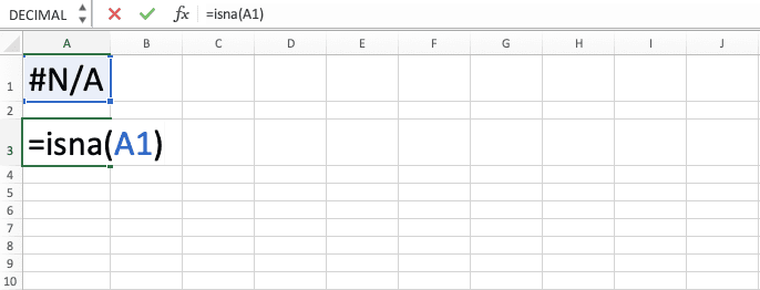
The general writing form of ISNA in excel is as follows.
= ISNA ( value )
The value input there is the data/formula we anticipate the #N/A error value from. We usually input a lookup formula in ISNA, such as VLOOKUP, HLOOKUP, or MATCH. That is because we almost always get a #N/A error value from these kinds of formulas.
Example of Its Usage and Result
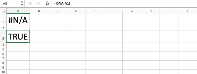
Here is an ISNA implementation and result example in excel.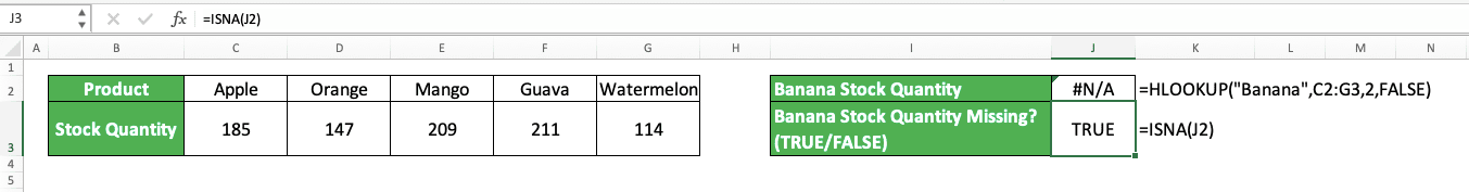
In this example, we use ISNA to identify the result of the HLOOKUP we write to get a banana stock quantity. For the identification process, we input the cell coordinate where we write our HLOOKUP to ISNA.
In the HLOOKUP reference table, there isn’t a banana stock quantity that our HLOOKUP wants to find. Thus, our HLOOKUP returns a #N/A error. Because of that, when we input the HLOOKUP result to our ISNA, we get a TRUE logic value from it.
Writing Steps
After discussing the ISNA writing form, input, and implementation example, now let’s discuss the steps to write it. As the ISNA writing form is quite simple, we only need to follow a few steps here to write ISNA completely.-
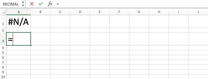
Type an equal sign ( = ) in the cell where you want to put your ISNA result in
-
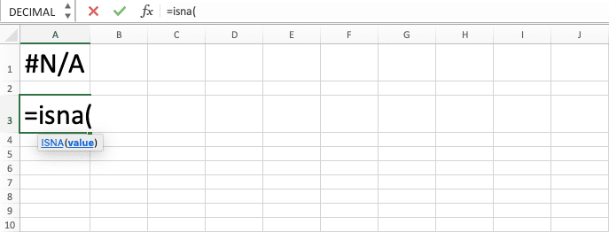
Type ISNA (can be with large and small letters) and an open bracket sign after =
-
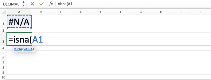
Input the data or the formula from which you want to identify the #N/A error value
-
Type a close bracket sign
- Press Enter
-
Done!
ISNA Combination with Other Formulas 1: IF ISNA VLOOKUP Yes No
As you may have already suspected, since the ISNA result is TRUE/FALSE, we usually combine its writing with another formula. Two of the formulas we usually combine with ISNA are IF and VLOOKUP.By combining ISNA, IF, and VLOOKUP, we can identify the availability of particular data and get value from the identification result. The value we produce from the formulas’ combination is often yes or no. We surely can produce other values besides yes or no. However, these values are often the standard ones we use.
Yes usually means the data is available and no usually means the data isn’t available. The general writing form of IF, ISNA, and VLOOKUP combination to produce this kind of result is as follows.
= IF ( ISNA ( VLOOKUP ( lookup_reference , reference_cell_range , result_column_index , lookup_mode ) ) , “No” , “Yes” )
We input our VLOOKUP to ISNA so ISNA can identify the VLOOKUP result, whether it is #N/A or not. If it is #N/A, then we set our IF to produce a “No” text. Otherwise, we set our IF to produce a “Yes” text.
Here is the implementation example of the IF, ISNA, and VLOOKUP combination to produce yes or no in excel.
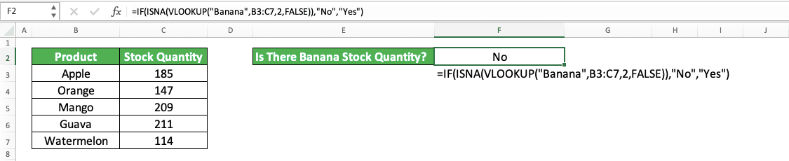
As you can see in the example, we get a “No” from the IF, ISNA, and VLOOKUP combination we write.
That is because our VLOOKUP doesn’t find the data we want and that makes ISNA produces TRUE. This, in turn, makes IF produce its TRUE result, which is a “No”.
ISNA Combination with Other Formulas 2: IF ISNA MATCH
Another ISNA formulas combination we might use is IF ISNA MATCH.The function of MATCH is to find the row/column position of data we want to find. Therefore, in a way, the result we get from IF, ISNA, and MATCH combination is similar to IF, ISNA, and VLOOKUP. You can think of IF, ISNA, and MATCH combination as an alternative to the IF, ISNA, and VLOOKUP.
Here is the three formulas’ combination writing form if we also use “Yes” or “No” as our final result.
= IF ( ISNA ( MATCH ( lookup_value , cell_range , [ match_type ] ) , “No” , “Yes” )
If we use MATCH instead of VLOOKUP, remember that MATCH can only process one row/column cell range. If we input a cell range larger than one row/column, then our IF can produce a #N/A error!
Make sure also that we input a direct lookup value to our MATCH. That means if we want to find a banana stock quantity, then we should input the stock quantity to MATCH. Inputting “Banana” like in a VLOOKUP will surely make our MATCH produces a #N/A error.
Here is the implementation example of IF, ISNA, and MATCH formulas combination in excel. We use “There Is” and “There Isn’t” as our IF result.
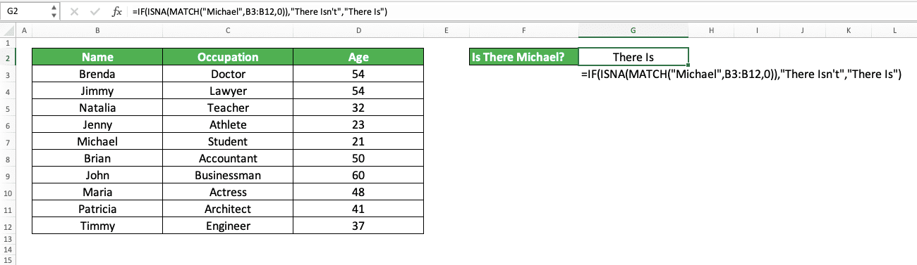
As you can see in the example, we get “There Is” from our IF, ISNA, and MATCH combination. That is because the data we want to find using MATCH, “Michael”, is available in the name column of the table.
As we want to find our data in the name column, we input this column cell range into our MATCH. We also input 0 in the MATCH because we want to find an exact match for the data we look up.
Our MATCH produces the “Michael” row position in the name column. As our MATCH doesn’t produce a #N/A error, that makes our ISNA produces FALSE. This causes our IF to produce its FALSE result as the final result, which is “There Is” in the example.
Identify All Types of Errors: ISERROR
Want to produce a TRUE logic value for all types of error not just a #N/A error? If that is what you need, then don’t use ISNA to help you identify your data/formula value. Use ISERROR instead.ISERROR will produce TRUE for any type of error that its input has. The general writing form of ISERROR in excel is similar to ISNA.
= ISERROR ( value )
Just input the data/formula which value you want to examine to ISERROR. ISERROR will produce TRUE if the data/formula has an error value!
For a better understanding of ISERROR, here is its implementation example in excel. We will compare its implementation result with ISNA too so you can see their differences clearly.
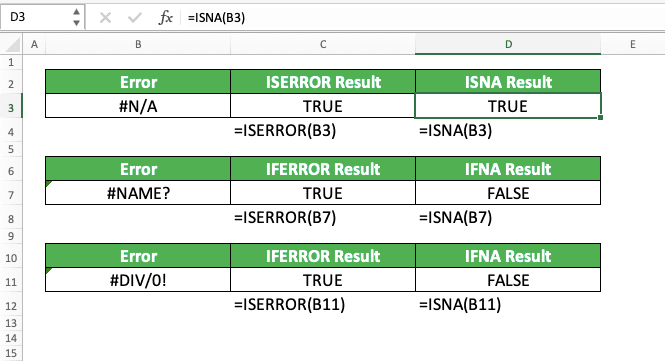
In the example, we input the same error value to ISERROR and ISNA in each row.
As you can see, ISERROR produces TRUE for all error values we input in it. Meanwhile, ISNA only produces TRUE for the #N/A error while it produces FALSE for other error values. That is because it can only identify the #N/A error.
Therefore, if you need to identify all error values in your formula, not just #N/A, use ISERROR instead of ISNA!
Exercise
After you have learned how to use the ISNA excel formula completely, now let’s do an exercise. This is so you can understand the tutorial lessons more practically!Download the exercise file and do all the instructions. Download the answer key file to check your answers if you have finished the exercise and want to check your answers. Or, probably, if you are confused about how to do the instructions
Link to the exercise file:
Download here
Instructions:
Use ISNA to do all the instructions!- Fill column no. 1 cells with TRUE/FALSE. The logic value depends on whether the parallel cell in column 1 contains #N/A or a number!
- Fill column no. 2 cells with V or X. The fill depends on whether the parallel cell in column 2 contains #N/A or a number! Use IF together with ISNA to do this instruction!
- Sum the parallel cell values in columns 1, 2, and 3. If there is a cell that contains a #N/A error, then assume it is 0 in the sum process! Use IF together with ISNA to do this instruction!
Link to the answer key file:
Download here
Additional Note
As ISNA only produces a TRUE/FALSE logic value, you almost certainly use it within an IF formula in excel.Related tutorials you should learn: