How to Use the ISERROR Formula in Excel: Functions, Examples, and Writing Steps
Home >> Excel Tutorials from Compute Expert >> Excel Formulas List >> How to Use the ISERROR Formula in Excel: Functions, Examples, and Writing Steps


In this tutorial, you will learn how to use the ISERROR function/formula in excel completely.
When processing data in excel, we sometimes need to identify whether we have made errors in the formulas we write. ISERROR can help you to do that cleanly.
Want to know more about this ISERROR function and how to use it optimally in excel? Read this tutorial until its last part!
Disclaimer: This post may contain affiliate links from which we earn commission from qualifying purchases/actions at no additional cost for you. Learn more
Want to work faster and easier in Excel? Install and use Excel add-ins! Read this article to know the best Excel add-ins to use according to us!
Table of Contents:
- What is the ISERROR formula in excel?
- ISERROR function in excel
- ISERROR result
- Excel version from which we can start using ISERROR
- The way to write it and its inputs
- Example of its usage and result
- Writing steps
- Get certain result if error: IF ISERROR
- Anticipate error from VLOOKUP: IF ISERROR VLOOKUP
- IF ISERROR alternative: IFERROR
- Exercise
- Additional note
What is the ISERROR Formula in Excel?
The ISERROR formula in excel is a formula that can identify whether our data/formula is an error or not.ISERROR Function in Excel
We can use ISERROR to help us know whether our excel formula produces an error or not.ISERROR Result
The result of an ISERROR formula is a TRUE or FALSE logic value, depending on the data or the result of the formula we input into it.Excel Version from Which We Can Start Using ISERROR
We can start using ISERROR in excel since excel 2003.The Way to Write It and Its Inputs
Here is the general writing format of an ISERROR formula in excel.
= ISERROR ( data_or_formula_to_evaluate)
The only input we need to give to ISERROR here is the data or formula we want to evaluate whether it has an error value or not. We almost always input a formula in ISERROR instead of data.
Example of Its Usage and Result
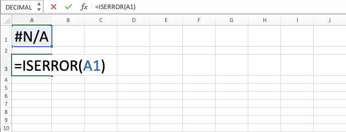
Here is an implementation example of ISERROR in excel.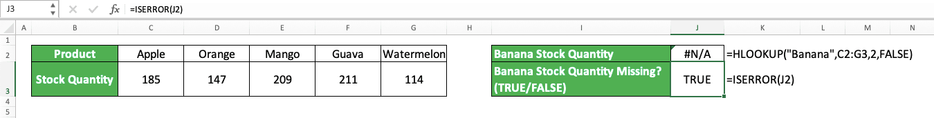
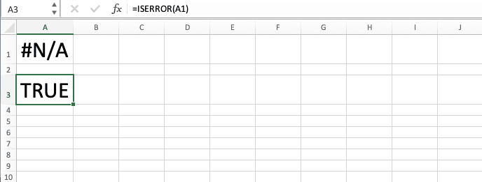
In the example, we look up specific data (banana stock quantity) in a table by using HLOOKUP and we get an error because the data is not there. As you can see, ISERROR can identify this error and gives us a TRUE logic value as a result.
If the data is there and the HLOOKUP gives us the banana stock quantity, our ISERROR formula will give a FALSE logic value instead.
Writing Steps
Now that you have learned the ISERROR formula writing format and implementation example, it is time to learn the detailed steps to write it. The writing steps are easy to understand because this function is simple and only needs one input to run-
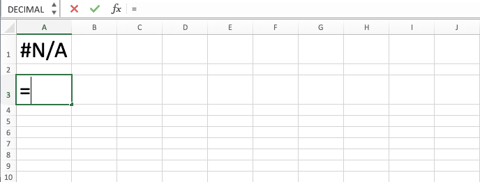
Type an equal sign ( = ) in the cell where you want to put the result in
-
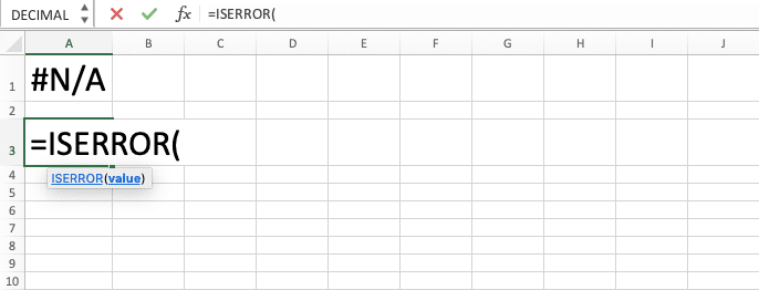
Type ISERROR (can be with large and small letters) and an open bracket sign after =
-
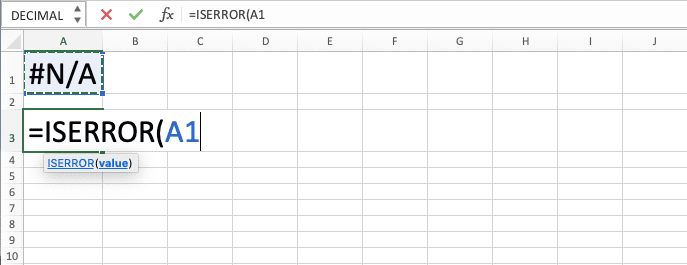
Input the data or the formula that you want to evaluate whether it has an error value or not after the open bracket sign
-
Type a close bracket sign
- Press Enter
-
Done!
Get a Certain Result if Error: IF ISERROR
If you use the ISERROR function in excel, you most likely don’t use it as the only function in your formula. More often than not, you will combine it with another function. That other function is most likely an IF.As ISERROR only produces a TRUE or FALSE logic value, IF can help you to get another result depending on whether the data or formula you evaluate produces an error or not. The way to combine ISERROR and IF to do something like that is as follows.
= IF ( ISERROR ( data_or_formula_to_evaluate ) , result_if_error , result_if_not_error )
Put the ISERROR formula as the logic condition of the IF. Then, input the result you want if what you evaluate with your ISERROR is indeed an error and another result if it isn’t.
To better understand the two functions combination, here is an implementation example.
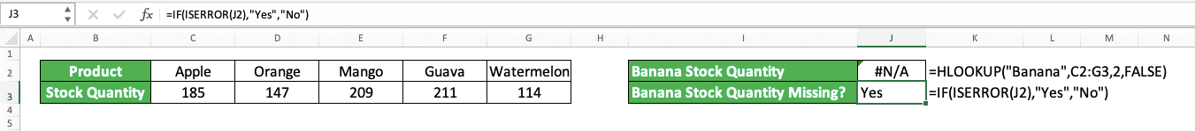
In the example, we want to get “Yes” or “No” instead of TRUE or FALSE to indicate whether the banana stock quantity is missing from the table on the left. For that, we input the ISERROR formula that evaluates the HLOOKUP that searches for the stock quantity data in our IF, followed by “Yes” and “No” as the TRUE and FALSE results of the IF.
By doing that, we get the result that we want from our data check.
Anticipate Error from VLOOKUP: IF ISERROR VLOOKUP
One of the most popular functions in excel is probably VLOOKUP. There can be instances when the VLOOKUP formula we write produce an error and we have to anticipate that. For this, we can combine the VLOOKUP with the IF and ISERROR combination.Here is the general writing format of the three functions combined in a formula.
= IF ( ISERROR ( VLOOKUP ( lookup_value , table_array , col_index_num , [ range_lookup ] ) ) , result_if_error , result_if_not_error )
Just input the VLOOKUP formula into the ISERROR formula to check whether it produces an error. The IF will then give us a final result depending on the error check result by the ISERROR formula.
Here is an implementation example of the formula.

As you can see above, we can anticipate the error from a VLOOKUP formula by putting it into the IF and ISERROR combination. The result is we can tell whether there is data for the banana stock quantity in the table or not.
IF ISERROR Alternative: IFERROR
If you use excel 2007 or newer and want to combine IF and ISERROR to give you a specific result when you find an error, you can use the IFERROR function instead to be much more straightforward in your formula writing.Here is the general writing format of an IFERROR formula in excel.
= IFERROR ( data_or_formula_to_evaluate , result_if_error )
IFERROR needs two inputs, the data or formula you want to evaluate whether its value is an error or not and the result if it is indeed an error. If there is no error, IFERROR will return to us the data or the formula result. This can become handy when we want to do just that, only change the data or the formula we input if we find an error.
Here is an IFERROR implementation example and its comparison with IF ISERROR.
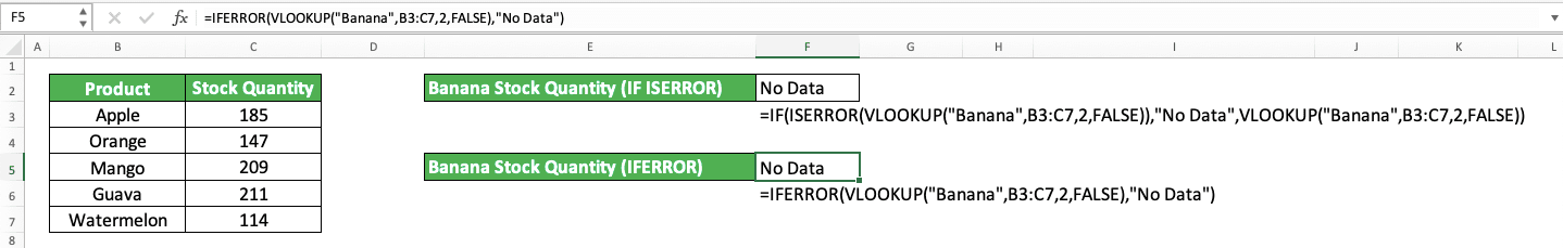
The IF ISERROR and IFERROR formulas above will produce the same result, either the VLOOKUP result or “No Data”. However, as you can see, the IFERROR formula writing is cleaner, simpler, and more straightforward than the IF ISERROR one.
Thus, if it fits you and the result you want, you can use IFERROR instead of IF ISERROR.
Exercise
After you have learned how to use the ISERROR formula in excel, now is the time you do an exercise to deepen your understanding!Download the exercise file below and do all the instructions. Download the answer key file to check your results if you have done the exercise or if you are confused about how to do it.
Link to the exercise file:
Download here
Instructions
Use ISERROR and IF to do all the instructions below- Mark the cell contents in column A with “Must Be Fixed A” or “Good” with the marks written in column no. 1!
- Mark the cell contents in column B with “Must Be Fixed B” or “Good” with the marks written in column no. 2!
- Mark the cell contents in column C with “Must Be Fixed C” or “Good” with the marks written in column no. 3!
Link to the answer key file:
Download here
Additional Note
ISERROR is one of the IS functions in excel. You can use these IS functions to check whether your data or formula has a certain type of value or not.Related tutorials you might want to learn too: