LOOKUP Excel Formula


In this tutorial, we will learn the use of the LOOKUP excel formula. LOOKUP formula in excel is useful to find data based on the approximate of your lookup value.
Two input sets can be used for this formula. The two of them will be explained deeper in the next parts of this tutorial.
Why do We Need to Learn Excel Look Up Function?
In the data processing on a spreadsheet file, sometimes we need to search based on the approximate of a certain value. Maybe for the process, we need a fast way to get the search result from a column/row/array. Doing it manually is hard because usually the reference column/row/array is large and there is much data to find. To solve this need, we should understand the automatic ways to do the search process.
The illustration of the search process needs in our work is when the assessment of salespeople performance in a company. Maybe we have determined the final mark ranges for the performance assessment based on the sales numbers. There can be many ranges for this final mark so it is difficult to determine it for each salesperson manually. If we do this assessment process in a spreadsheet file, then using a formula will make it more accurate and easier.
For that, you should learn how to use the LOOKUP excel formula. LOOKUP excel formula can easily find data based on estimation in your column/row/array. It is important to understand especially if you often deal with the search process in your spreadsheet file. This function can be an alternative way to find your data you need as fast as possible.
What is the LOOKUP Excel Formula?
LOOKUP excel formula is a formula to get something from a data approximate which is searched in a column/row/array. It is one of the search formulas available in this software besides VLOOKUP, HLOOKUP, INDEX MATCH, and others.
Approximate in here means the smaller and nearest one to your search reference data. But, if there is an exact match, then that match will be made the base for the result.
There are two sets of inputs that can be used in the LOOKUP excel formula. In general, the two sets of inputs can be explained briefly as follows:
First input set:
=LOOKUP(lookupvalue, lookupvector, [resultvector])
Notes:
- lookupvalue = reference value to be found the more or less of
- lookupvector = the column/row where the more or less will be searched in
- resultvector = optional. The place where the result of the formula will be had
Second input set:
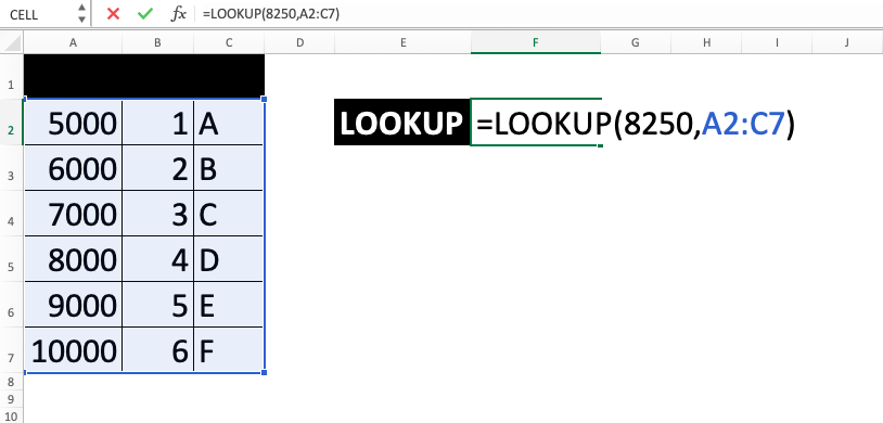
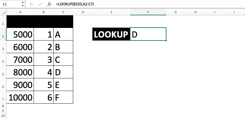
=LOOKUP(lookupvalue, array)
Notes:
- lookupvalue = reference value to be found the more or less of
- array = array where the search process will be conducted
How to Use This Formula to Lookup Value in Excel?
The following will explain how to use the LOOKUP excel formula. The explanation will be divided into two as there are two sets of inputs that can be used in it. The first input set does its process in columns/rows while the second input set does it in an array. Choose which method and input set you want to use based on your data processing need!
It is important to remember that the column/row where your reference value is searched must be sorted in ascending order (A to Z for text). If it is not ordered like that, then the search process can produce a wrong or error result.
Using LOOKUP Function in Excel
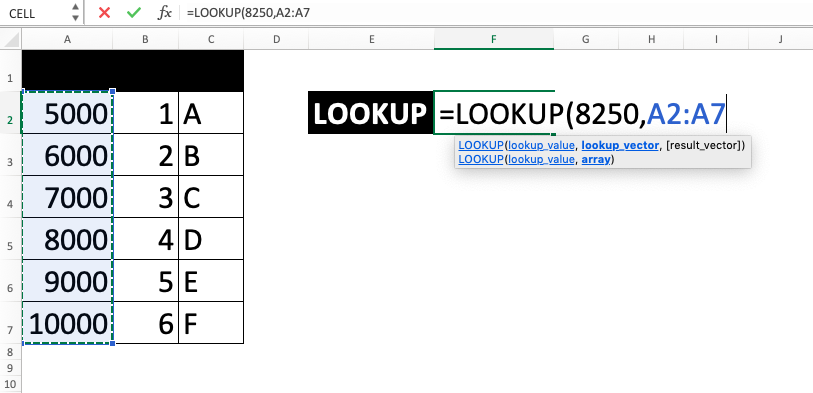
Method 1: First Input Set
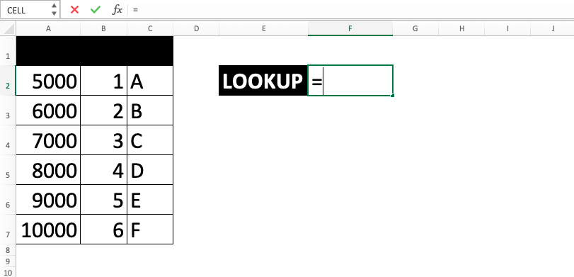
-
Type equal sign ( = ) in the cell where you want to put the result

-
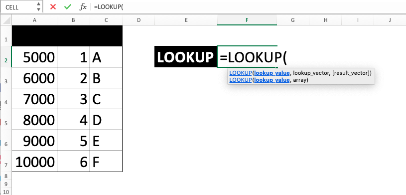
Type LOOKUP (can be with large and small letters) and open bracket sign after =

-
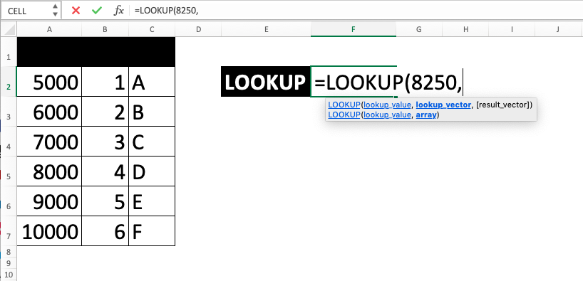
Input the search reference value or cell coordinate where that value is. Then, type a comma sign ( , )

-
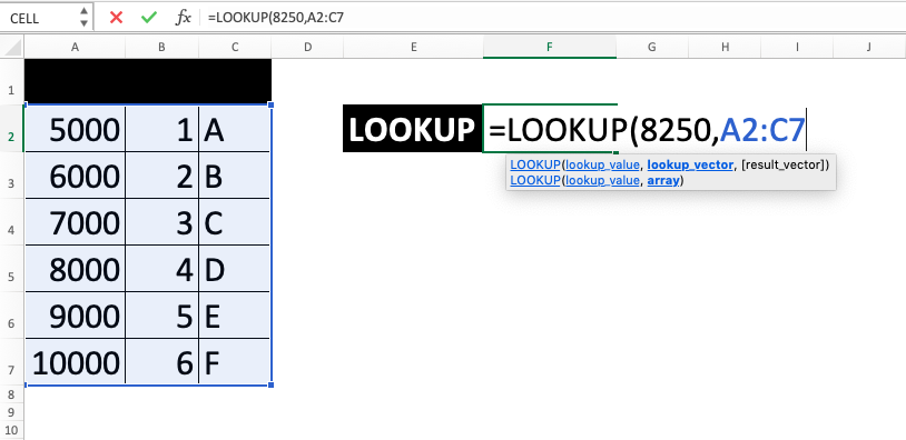
Drag cursor on the column/row cell range where the search of the approximate (less and nearest) of your reference value will be done. Make sure the data in it is already in ascending order (A to Z for text). If it is unordered, then it can make your result wrong/error
-
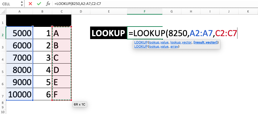
Optional: If the result you want to get is not in the previously inputted cell range, then do this. Type a comma sign then input the column/row cell range where that result is. The result will be taken in the parallel position of where the approximate of your reference value is found. Because of that, make sure the column/row cell range here is in line with the reference column/row cell range
-
Type close bracket sign
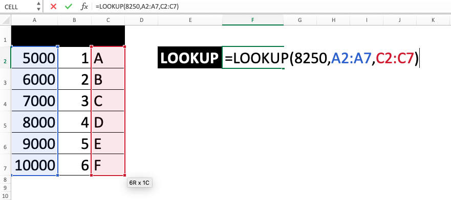
- Press Enter
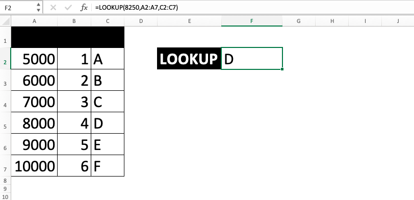
-
The process is done!
Method 2: Second Input Set
-
Type equal sign ( = ) in the cell where you want to put the result
-
Type LOOKUP (can be with large and small letters) and open bracket sign after =
-
Input the search reference value or cell coordinate where that value is. Then, type a comma sign ( , )
-
Drag cursor on the array cell range where the search process will be done. Your reference value approximate will be done on the first column/row of the array. Whereas the result will be had from the last column/row of the array in the parallel position of your reference.
Don’t forget to make sure the data where your reference is searched is already in ascending order (A to Z for text). If it is unordered, then it can make your result wrong/error
-
Type close bracket sign
- Press Enter
-
The process is done!
Exercise
After you have learned how to use the LOOKUP excel formula with the two input sets, now let’s do an exercise. This is done so you can deepen your understanding of the steps earlier.
Download the exercise file and answer all the questions. Download the answer key file if you have done the exercise and want to check your answers. Or probably when you are confused about how to answer the questions!
Link to the exercise file:
Download here
Questions
Use the LOOKUP excel formula to answer all the questions!- In which minimum score is 74? Use the first input set!
- In which letter is the 74? Use the first input set!
- In which level is the 74? Use the second input set!
Link to the answer key file:
Download here
Additional Notes
- If the reference value is larger than all data in the searched column/row, the approximate is the largest one
- If the reference value is smaller than all data in the searched column/row, it will be an #N/A error
- The LOOKUP excel formula is not case sensitive