How to Use VLOOKUP from Another Sheet
Home >> Excel Tutorials from Compute Expert >> Excel Formulas List >> How to Use VLOOKUP from Another Sheet


In this tutorial, you will learn how to use the VLOOKUP formula if its reference table is in another sheet.
Before learning from this tutorial, you need to understand the basics of using VLOOKUP in excel first. If you haven’t understood it, you can learn it here.
VLOOKUP is a data lookup formula often used by excel users. Sometimes, the reference table where it looks for its data is in a different sheet from where you write your VLOOKUP.
We need some tweaks when using VLOOKUP so it can function in this situation as well. We will discuss in detail what are those tweaks needed.
Disclaimer: This post may contain affiliate links from which we earn commission from qualifying purchases/actions at no additional cost for you. Learn more
Want to work faster and easier in Excel? Install and use Excel add-ins! Read this article to know the best Excel add-ins to use according to us!
Table of Contents:
- The way to write it and its inputs
- Example of its usage and result
- Writing steps
- An alternative way: use the excel define name menu
- VLOOKUP from another sheet and another file
- VLOOKUP with more than one sheet references and one-by-one lookup method
- VLOOKUP with a dynamic sheet reference
- Complete VLOOKUP lesson and other use cases
- Exercise
- Additional note
The Way to Write it and Its Inputs
Generally, the VLOOKUP writing that has a reference table in a different sheet is as follows.
=VLOOKUP(lookup_value, ’sheet_name’!table_array, col_index_num, [range_lookup])
And here is a brief explanation for each element of the writing inputs.
- lookup_value = the lookup reference value of your VLOOKUP
- sheet_name = the sheet name where your reference table is and where VLOOKUP will look for your data
- table_array = the cell range where your reference table is, in that other sheet
- col_index_num = the left-to-right order of the column where your VLOOKUP result should be taken
- [range_lookup] = an optional input. Your VLOOKUP search mode, whether it must be an exact match with your lookup reference value or it can be approximate. Input TRUE for approximate and FALSE for exact. Its default value is TRUE
Example of Its Usage and Result
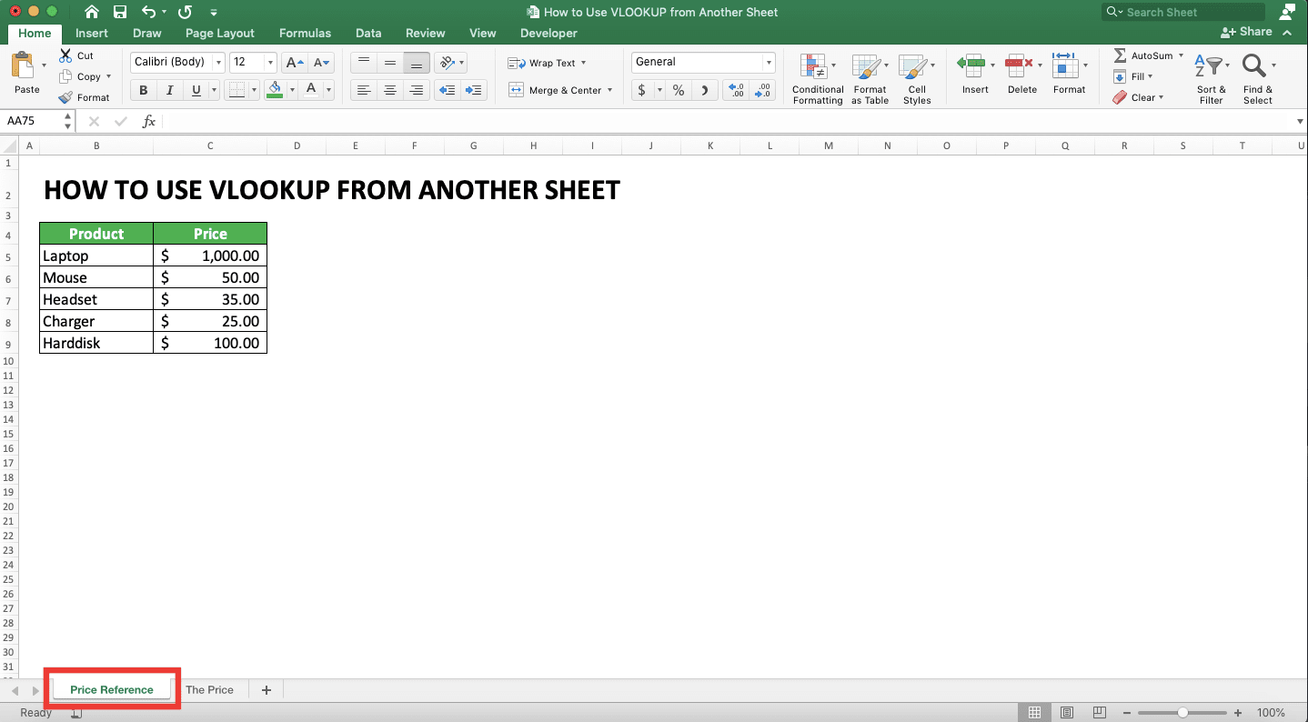
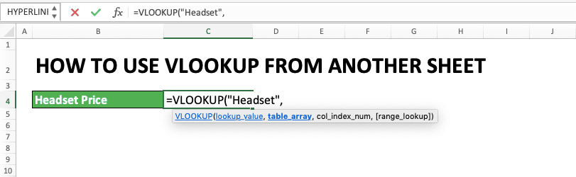
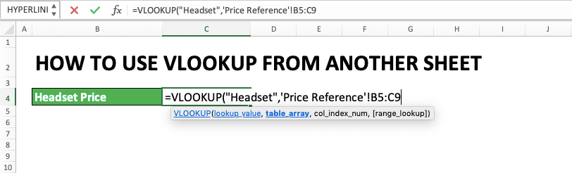
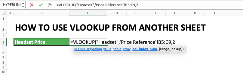
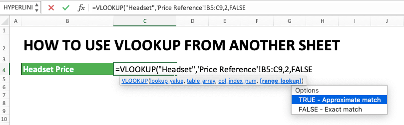
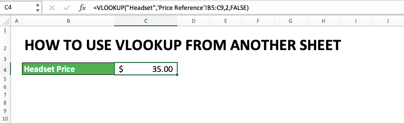
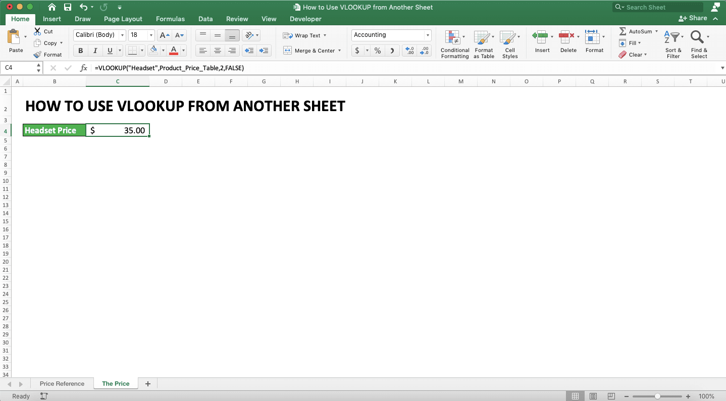
The following will give and explain the example of different sheet VLOOKUP usage and result.First, we can see here that the reference table is in a different place with the VLOOKUP writing (the reference table is in the “Price Reference” sheet and the VLOOKUP writing is in the “The Price” sheet).
And to refer to this data table, we do it like what you can see in the following screenshot’s formula bar.
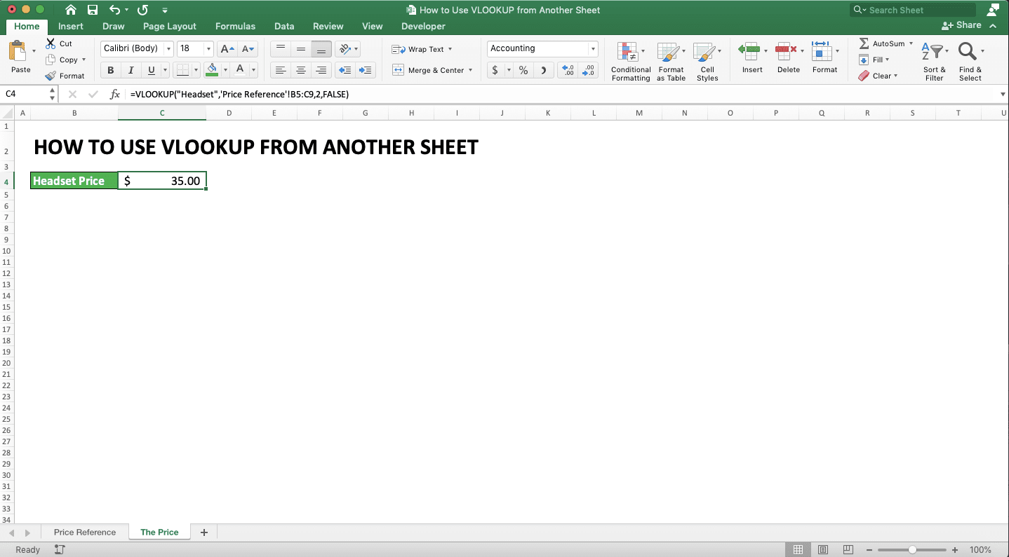
You can see there how the VLOOKUP formula writing follows the pattern explained in the previous part. The difference with the normal VLOOKUP writing is there are sheet name and exclamation mark (!) before the reference table cell range.
Besides that difference, other input writings are still the same. By giving your inputs like that, you will get the different sheet VLOOKUP result you need.
Writing Steps
How to do the VLOOKUP writing with a different sheet reference in detail? We will give here the steps and the writing example screenshots to help you learn.-
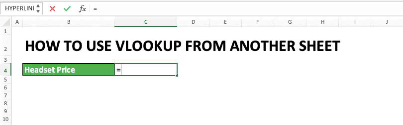
Type an equal sign ( = ) in the cell where you want to put your VLOOKUP result
-
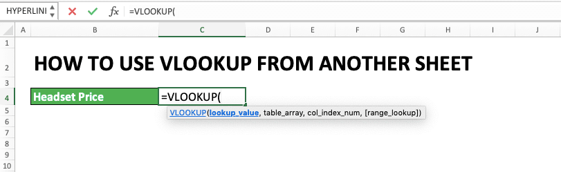
Type VLOOKUP (can be with large or small letters) continued with an open bracket sign
-
Input your lookup reference value or the cell coordinate where it is, then type a comma sign ( , )
-
Input the cell range where the reference table is in another sheet then type a comma sign. You can input it by clicking the sheet where the table is and drag your pointer on the table cell range.
After the dragging process is done, click again on the sheet where you write your VLOOKUP. The reference table’s sheet name and cell range are automatically inputted in your VLOOKUP!
You can also type the reference table cell range directly although it is troublesome. If you type it, don’t forget to type the sheet name first inside quotes sign ( ‘’ ) continued with an exclamation mark ( ! ). Only after that, you can type the reference table cell range.
-
Input the result column order in your reference table or the cell coordinate where the order number is
-
Optional: Type a comma sign, then input TRUE or FALSE for the VLOOKUP search mode you want. TRUE for the approximate search mode and FALSE for the exact search mode.
Don’t forget to sort your reference table’s first column in ascending order if you use TRUE. The default input here if there is no input given is TRUE
-
Type a close bracket sign

- Press Enter
-
Done!
An Alternative Way: Use the Excel Define Name Menu
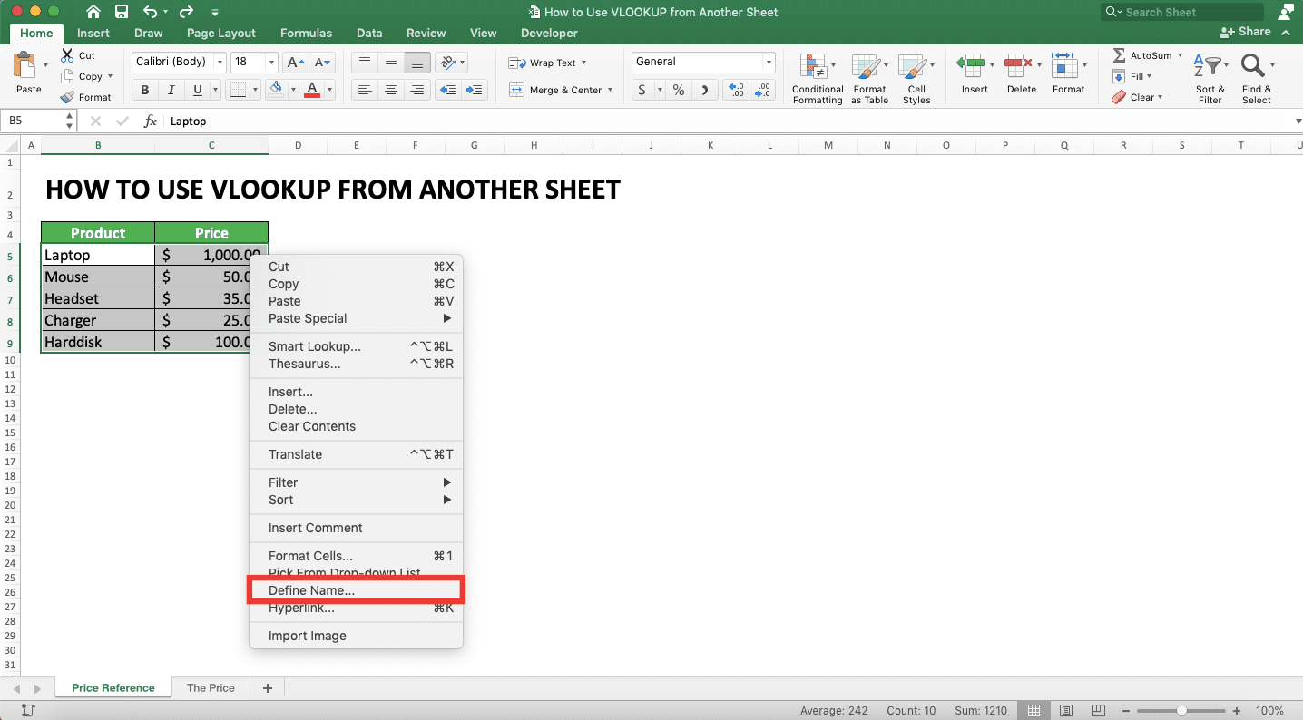
Don’t want to move around sheets when you type your VLOOKUP formula? You can give a name to your reference table cell range so you don’t have to do that. After giving the name, you just need to refer to that name when giving the reference table input in your VLOOKUP.The name itself can be given by using the excel Define Name menu. Highlight the cell range where your reference table is, right-click, and choose Define Name….
In the dialog box shown, input the name you will refer to when you use the reference table in your formulas. Note that the name you give cannot have spaces in it. After giving the name, click OK.
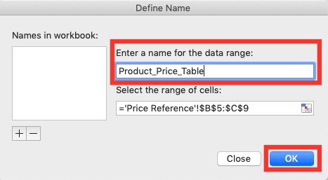
Your cell range naming is done!
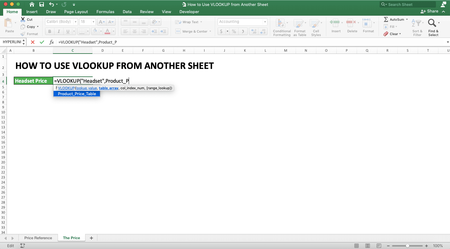
If you want to use the name, then you just need to type it when you need it. In the VLOOKUP context, that means you input the name when you need to input your reference table’s cell range.
Generally, the writing form of this can be illustrated as follows.
=VLOOKUP(lookup_reference_value, reference_table_name, result_column_order, [search_mode])
As seen above, the difference with the standard different sheet VLOOKUP writing is just in the reference table input. The cell range input is changed with the reference table name you have saved before.
The name you have saved will also show up in excel suggestions when you begin typing it.
Do the reference table’s name input correctly and your VLOOKUP result will be there!
VLOOKUP from Another Sheet and Another File
What if your reference table isn’t just in a different sheet but also in a different table?The basic is actually almost the same as VLOOKUP with different sheet but the same file. It is just you need to add the workbook file name in the reference table input if the file is opened. If the table file is closed, you need to add the file path too before the workbook file name.
This can be inputted automatically if you go to your reference table’s file and sheet when you input your VLOOKUP. Do the pointer drag on the table’s cell range so the input will be automatically given in your VLOOKUP.
Generally, the writing of the different sheets, different file VLOOKUP, if the table file is opened ,can be seen below.
=VLOOKUP(lookup_reference_value, ’[workbook_name]sheet_name’!reference_table_cell_range, result_column_order, [search_mode])
And if the table file is closed, then the writing becomes like this.
=VLOOKUP(lookup_reference_value, ’file_path[workbook_name]sheet_name’!reference_table_cell_range, result_column_order, [search_mode])
To make it clearer, see the following example.
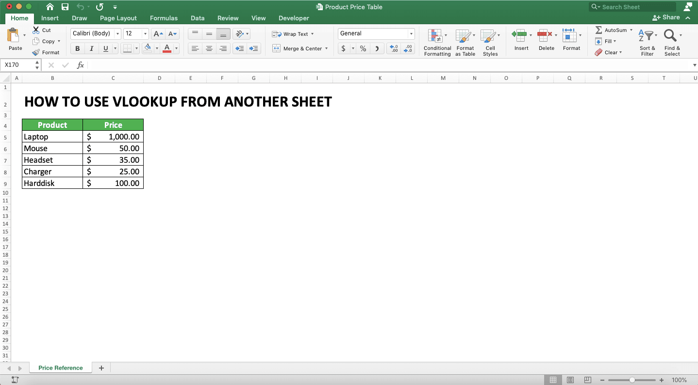
In the above example, there is a reference table in the “Price Reference” sheet of the “Product Price Table” file. How to refer to it in the VLOOKUP formula which is written in a different sheet?
You need to open both the VLOOKUP and reference table files first. Then, you drag on the reference table cell range when inputting your VLOOKUP’s reference table. The result will be like this.
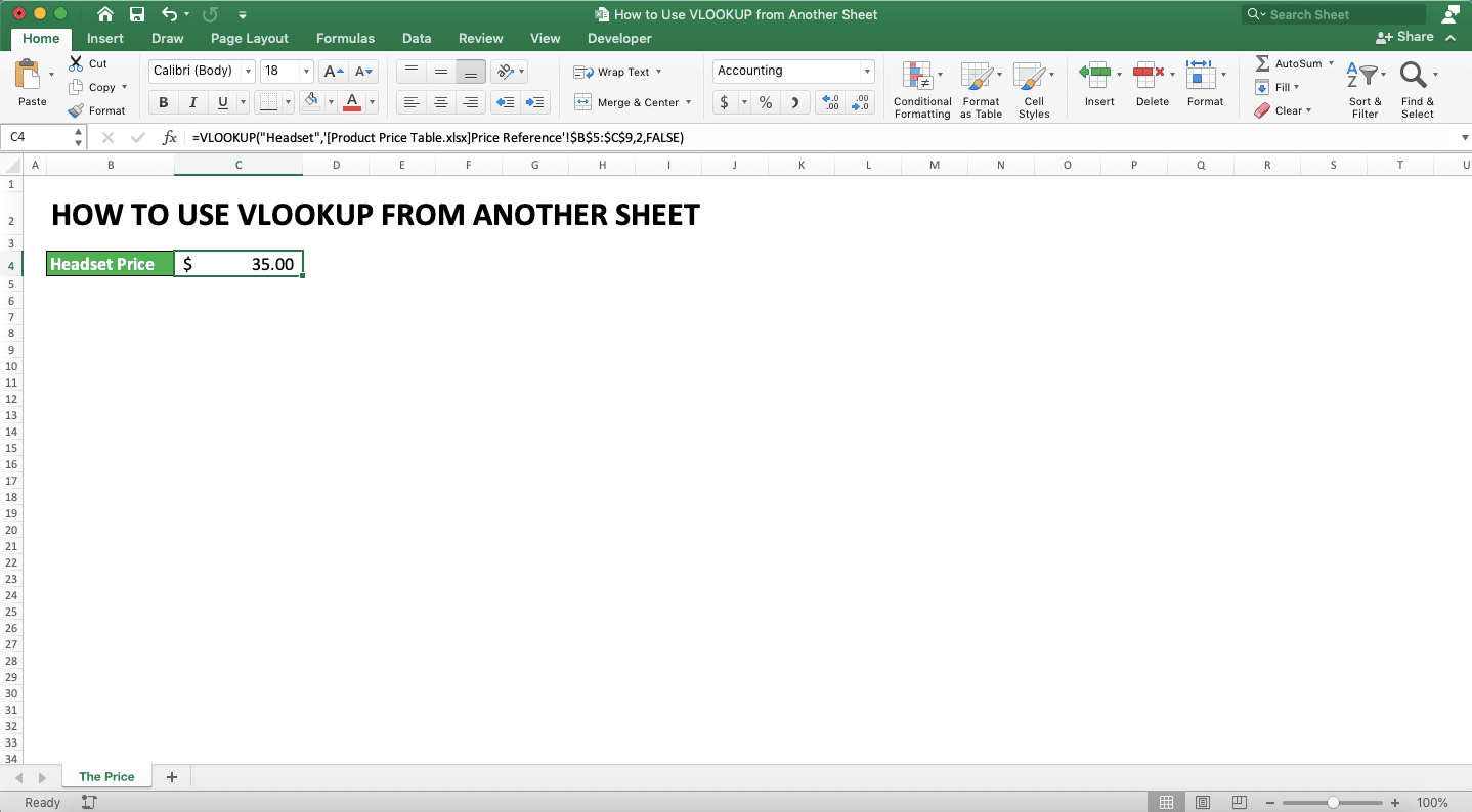
When the table file is closed, then its file path will be automatically added when you have inputted your table.
Give the inputs correctly and you will get your VLOOKUP result easily!
VLOOKUP With More Than One Sheet References and One-by-One Lookup Method
Maybe, there is a situation when there are multiple reference tables we want to input into our VLOOKUP. The data in those tables are different from one another and those tables are in different sheets too. We want if our data isn’t found in one table, then VLOOKUP will automatically look for the data in other tables.Can we do that? The answer is we can, by using the combination of IFERROR and VLOOKUP.
Generally, the IFERROR VLOOKUP writing to find data like that is as follows.
=IFERROR(VLOOKUP(lookup_reference_value, ’sheet_name_1’!reference_table_cell_range_1, result_column_order, [search_mode]), IFERROR(lookup_reference_value, ’sheet_name_2’!reference_table_cell_range_2, result_column_order, [search_mode],…, result_if_data_not_found)
In the writing, we can see that we need to make nested IFERROR VLOOKUPs. Write earlier the IFERROR VLOOKUP with the reference table input you want to look at first. Then, input your IFERROR VLOOKUP continuously until you have inputted all your reference tables.
In the IFERROR VLOOKUP’s last part, don’t forget to input the result if your data isn’t found in all reference tables.
As an illustration, here is an implementation example of the writing above and its result in excel.
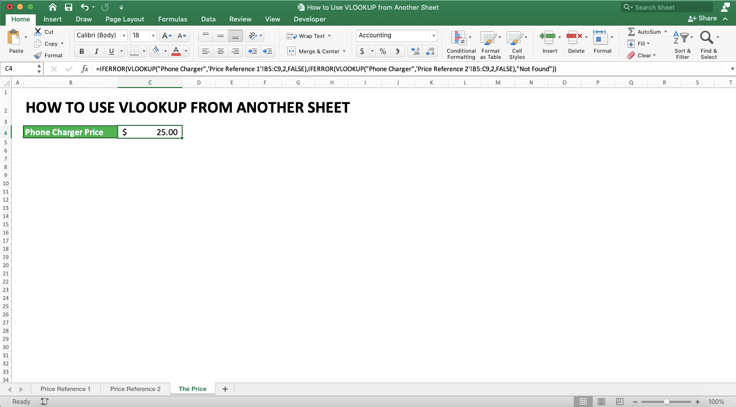
As seen in the example, there are two sheets with different reference tables. With that situation, then the VLOOKUP writing is as seen in the example’s formula bar.
In the process, VLOOKUP will look at the “Price Reference 1” sheet’s table first before looking at “Price Reference 2”. In this case, the product price we seek is found in the “Price Reference 2” sheet’s reference table
If we don’t find our lookup reference value on those two sheets, the formula will produce “Not Found” text as inputted.
If you need more than two reference tables, then just input IFERROR VLOOKUP as many as your reference tables.
VLOOKUP With a Dynamic Sheet Reference
What if there are multiple reference tables on different sheets and we want to find data based on a certain value? If the value is this, then the reference table is this. And if the value is that, then the reference table is that.In other words, we want our VLOOKUP reference table to have a dynamic sheet reference.
Can we do that using VLOOKUP? Of course, we can! For this, you need to combine your VLOOKUP with IF.
Generally, the VLOOKUP and IF combination is written as follows to have a dynamic sheet reference.
=VLOOKUP(lookup_reference_value, IF(logic_condition, ’sheet_name_1’!reference_table_cell_range_if_the_logic_condition_is_true…, ’sheet_name_2’!reference_table_cell_range_if_the_logic_condition_is_false), result_column_order, [search_mode])
As you can see, we input the IF formula in the reference table input part. Give a logic condition based on your needs and input the reference table if the logic is true and false. Input the nested IFs as long as you need if there are more than 2 reference tables.
The example of this VLOOKUP IF application is as follows.
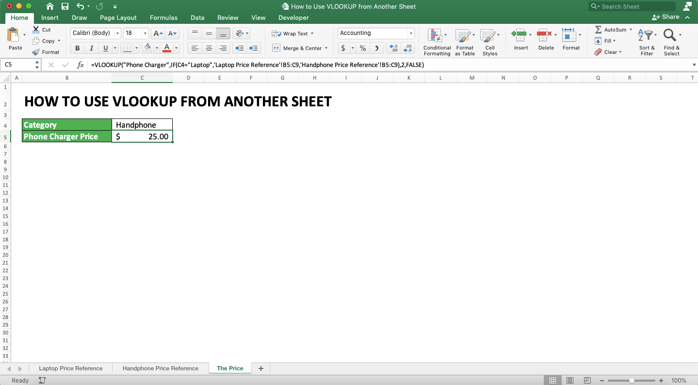
In the example, we determine the VLOOKUP reference table based on the category cell’s value. If the value is “Laptop” then the reference table must be had from the “Laptop Price Reference” sheet. If “Handphone”, then the reference table must be had from the “Handphone Price Reference” sheet.
With that condition, then the VLOOKUP’s reference table becomes what you see in the formula bar. The logic condition input in the IF is whether the category cell’s value is “Laptop” or not. The result if it is true is the “Laptop Price Reference” sheet’s reference table cell range. If false, then it becomes the “Handphone Price Reference” sheet’s reference table cell range.
That is the example if there are two reference tables on a different sheet. If there are more than 2, then you just need to input as many IF as you need.
Complete VLOOKUP Lesson and Other Use Cases
Want to learn other VLOOKUP use cases? Maybe you want your VLOOKUP’s lookup reference value to be more than 1? Or probably you want to find the second or third match for your VLOOKUP result?You can learn all that and more by reading parts of this complete VLOOKUP tutorial we have here!
Exercise
After you learn how to use VLOOKUP which uses a reference table from another sheet, now let’s do an exercise!Download the exercise file and answer all the questions. Download the answer key file if you have done the exercise and want to check your answers!
Link to the exercise file:
Download here
Questions
Answer these questions on the “Answer” sheet in the appropriate cells!- How many stocks of product C are there in the warehouse at the end of March? Use a standard different sheet VLOOKUP to answer it!
- How many product F sold in February? Use the IFERROR VLOOKUP combination to answer it by inputting March’s reference table first! Give a “Not Found” text if the data isn’t found!
- How many product A sold in the month of C4 cell’s value? Use the IF VLOOKUP combination to answer this by inputting February’s reference table as the true result!
Link to the answer key file:
Download here
Additional Note
If you need a more flexible lookup formula than VLOOKUP, use INDEX MATCH! Learn the formula in our complete tutorial here!Related tutorials you should learn too: