How to Write “Not Equal to” in Excel

In this tutorial, you will learn completely about how to write “not equal to” in excel.

When writing a formula, especially the one that requires criteria or logic conditions, we sometimes need to write “not equal to”. This is so we can get the correct result that we want for our data processing.

If we don’t know how to do it, then we cannot use the formula correctly to get what we need! Therefore, if you need to write “not equal to” but don’t know how, then you should learn from this tutorial.

Disclaimer: This post may contain affiliate links from which we earn commission from qualifying purchases/actions at no additional cost for you. Learn more

Want to work faster and easier in Excel? Install and use Excel add-ins! Read this article to know the best Excel add-ins to use according to us!

“Not Equal to” Symbol/Operator in Excel

In excel, “not equal to” is symbolized with what we call chevrons or angle brackets ( <> ).

The Way to Write “Not Equal to” in Excel

We can write a “not equal to” criterion/logic condition with a writing form like this generally.



For example, if we want to write “not equal to 5” in excel, then we can just write <>5. Or, if we want to write “not equal to John”, then we can just write <>John.

Pretty simple, isn’t it?

Just remember that if you use “not equal to” for a criterion, then you need to envelop the writing with quotes ( “” ). In the criterion, besides a text and number value, you need to add an ampersand symbol ( & ) between the <> and the value (e.g. not equal to cell B3 is written as “<>”&B3. Additionally, not equal to 12 November 2008 is written as “<>”&DATE(2008,11,12))

Example of Writing “Not Equal to” in a Formula 1: Excel IF Not Equal to

One of the formulas that may often use a “not equal to” writing is IF. That is because it has a logic condition input where you usually need to do comparison between one value and another.

How to write a logic condition input if you need to use the “not equal to” symbol? We can illustrate the general writing form of the IF with that caveat like this.



We put the <> symbol of “not equal to” between the value that we want to compare. If the values aren’t similar, then IF will produce its TRUE result. If the values are similar, then IF will produce its FALSE result.

We can see the implementation example of that IF writing below.



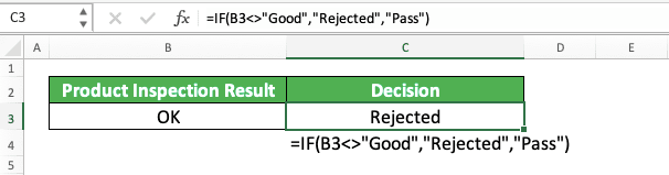
In the example, we try to see whether we accept a product or not after we get its inspection result. To determine the decision, we can use IF.

In here, anything that the inspection says not “Good” will be rejected (even though the inspection result is still “OK”). Because of that, we write the IF logic condition to be the product inspection result not equal to “Good”. We write it by using the form we discussed earlier, which in this case is B3<>”Good” (the inspection result data is in cell B3).



If it is TRUE, then we should reject the product and mark it with the word “Reject”. If it is FALSE, then we should pass the product and mark it with the word “Pass”.

As you can see, the logic condition works with that “not equal to” writing and the result is “Reject”!

An Example of Writing “Not Equal to” in a Formula 2: Excel SUMIF Not Equal to

What if we need a “not equal to” criterion in our SUMIF? How do we write that?

For this, the writing is quite the same as the one we do in the logic condition input of an IF. However, as we previously discussed, we must not forget to add quotes and ampersand symbols when they are needed.

The general writing form of SUMIF with a “not equal to” criterion is like this.



This SUMIF writing form is for if we pair up the “not equal to” symbol with a text or number. This is often the case when we need to use a “not equal to” criterion in SUMIF.

However, if the one we pair up isn’t a text or a number, then we write our SUMIF like this.



We add an ampersand after the “not equal to” symbol and the quotes. After the ampersand, we input the value we want the data to not equal to if we should sum their numbers.

We can also use both ways of “not equal to” criterion writing when we write the SUMIF formula sibling instead, SUMIFS.

To make the understanding clearer, take a look at the SUMIF with a “not equal to” criterion implementation example below.



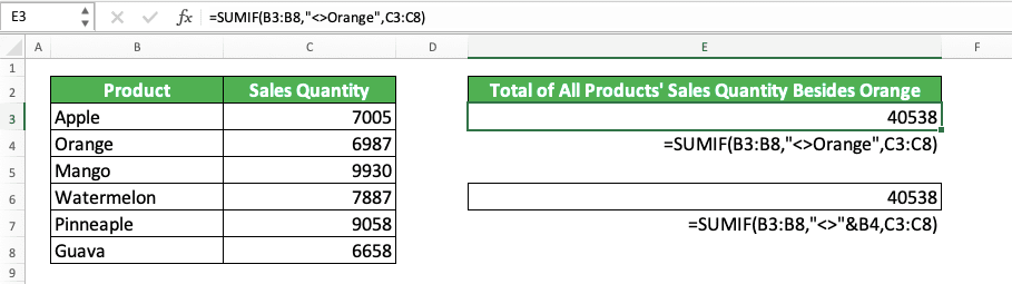
Here, we can see the writing of a “not equal to” criterion in SUMIF with a text value and cell coordinate. We want to sum the sales quantities of the products besides oranges and that can be done in those two ways.

For the “not equal to” criterion with the “Orange” text value, we write the SUMIF criterion as “<>Orange”. For the one with the cell coordinate, we write the SUMIF criterion as “<>”&B4 (B4 is the cell with an “Orange” text value in it).

As we can see in the example, we get the same results from both SUMIF writing! They are the product sales quantities total excluding the orange one.

An Example of Writing “Not Equal to” in a Formula 3: Excel COUNTIF Not Equal to

If we have to write a “not equal to” in COUNTIF, then the writing method is similar to SUMIF. That is in the way that we use it as a criterion input in COUNTIF too.

So, because of that, here is the general writing form of COUNTIF with a “not equal to” criterion.



That writing form is if the value you pair with the “not equal to” symbol is a text or number. If it is another type of value (or a cell coordinate), then the writing form becomes like this.



As with the SUMIF, you need an ampersand to connect the “not equal to” symbol with the comparison value.

To make the understanding clearer, here is the implementation example of both COUNTIF writing forms in excel.



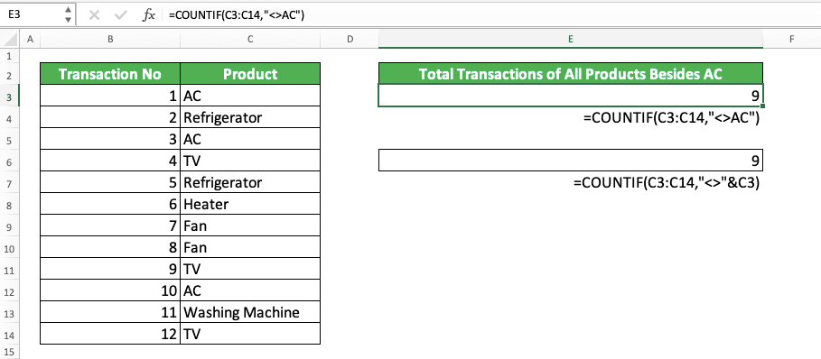
Here, we have data of transactions in a day in an electronic shop. We want to find out the number of transactions done if we exclude AC transactions from it.

To do this, we use COUNTIFs with a “not equal to” criterion. We can use both direct text typing or cell coordinate values to make the “not equal to” criterion.



If we use a direct text value, then we write the criterion as “<>AC” for the example. If we use a cell coordinate, then we write the criterion as “<>”&C3 (where an “AC” text is).

Using both ways of writing, we can find the number of transactions that exclude the AC ones!

“Not Equal to” Alternative: NOT and “Equal to”

You can also write a “not equal to” in excel using the combination of NOT and “equal to”. That is because “equal to” is the opposite of “not equal to” and NOT can reverse our logic value in excel.

We symbolize an “equal to” with an equal symbol ( = ) in excel. Here is the general writing form of NOT and “equal to” which is the same with a “not equal to”.



In the writing form, we pair two values that we want to compare using an equal symbol. The resulting logic value from the comparison will be reversed by NOT. That way, we will get the same logic value as if we use a “not equal to” writing there!

As a note, however, you cannot use NOT and “equal to” to represent “not equal to” in a criterion. For that, you have to use normal “not equal to” writing.

To give you an implementation example of this NOT and “equal to”, look at the screenshot below.



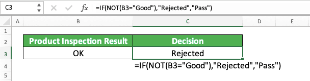
We use the same example like the one we use to illustrate IF with a “not equal to” logic condition. We can see that both of NOT with “equal to” and “not equal to” methods get the same results!

For the IF logic condition input here, we pair the product inspection result data and “Good” using an equal symbol. This produces a TRUE if the product inspection result is “Good” and FALSE if otherwise.

After that, we envelop the “equal to” logic condition with NOT. This reverses the “equal to” logic condition result (TRUE becomes FALSE and FALSE becomes TRUE). Thus, it becomes similar as if we use a “not equal to” logic condition!

IF then will produce its result based on what NOT gives it. In the example, our NOT gives FALSE. Thus, IF gives its FALSE result, which is “rejected”.

Exercise

After we have learned how to write “not equal to” in excel, now let’s do an exercise. This is so we can practice what we have learned and understand the tutorial material deeper.

Download the exercise file and answer all the questions below. Download the answer key file if you have done the exercise and want to check your answers. Or probably when you are stuck with one or more questions!

Link to the exercise file:
Download here

Instructions

Answer each question using the excel “not equal to” writing in the appropriate cell!

1. How many products in the “Most Products Sold” column are not an apple?
2. What is the monthly sales quantities total, excluding for the months where mango is the most sold product?
3. Check the most sold product in June! If the most sold product is apple, then fill the cell with “Apple Again”. If not, then fill it with “Not Apple”!

Link to the answer key file:
Download here

Additional Note

In its comparison process, the “not equal to” symbol is not case sensitive.



Other tutorials you should learn: