How to Use the EXACT Function in Excel: Usabilities, Examples, and Its Writing Steps
Home >> Excel Tutorials from Compute Expert >> Excel Formulas List >> How to Use the EXACT Function in Excel: Usabilities, Examples, and Its Writing Steps


In this tutorial, you will learn how to use the EXACT function in excel completely.
When working in excel, we sometimes need to compare the text we have and produce a result based on that. We can use EXACT to help us do the comparison process and get an accurate result from it.
Want to know more about this formula and how to utilize it optimally in excel? Read this tutorial until its last part!
Disclaimer: This post may contain affiliate links from which we earn commission from qualifying purchases/actions at no additional cost for you. Learn more
Want to work faster and easier in Excel? Install and use Excel add-ins! Read this article to know the best Excel add-ins to use according to us!
Table of Contents:
What is the EXACT Function in Excel?
EXACT function in excel is a function that can help us to compare two texts in a case-sensitive manner.EXACT Usabilities
You can use EXACT to get the comparison result of two texts in excel. The application of EXACT will become something like a logic condition in excel. Because of this, we use EXACT mainly with another formula that works with logic conditions, like IF.EXACT Result
The result EXACT gives us is a TRUE or FALSE logic value. If the two texts we compare with EXACT are similar, then EXACT will give us TRUE. If they aren’t the same, then it will give us FALSE.Excel Version from Which We Can Start Using EXACT
We can start using EXACT in excel since excel 2003.The Way to Write It and Its Inputs
Here is the general writing form of EXACT in excel.
= EXACT ( text1 , text2 )
When writing EXACT, we just need to input the two texts we want to compare with the formula.
Just so you know, we can input other types of data besides text to EXACT. However, we usually use it to compare text since it is case-sensitive in its comparison process. This case-sensitive nature is something we cannot get if we just compare our data using an equal sign ( = ).
Example of Its Usage and Result
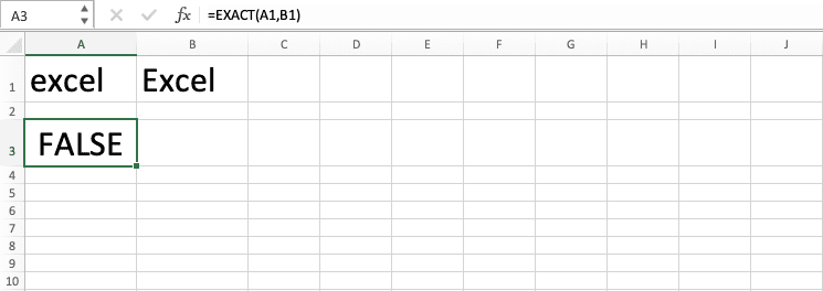
Here is the implementation example of the EXACT formula in excel.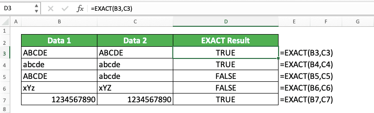
As you can see here, EXACT compares the two texts we input into it in a case-sensitive manner. It only gives us TRUE if the two texts are similar in content and letter cases. If the two texts are different in letter cases, even though the content is the same, EXACT will give us FALSE.
EXACT can also compare data that aren’t text. As you can see in the last row of the example, it returns TRUE when it compares similar numbers.
Writing Steps
After we discussed the EXACT writing form, inputs, and implementation example, now let’s discuss its writing steps. You should be able to understand these steps quite easily since EXACT only needs two simple inputs in its writing.-
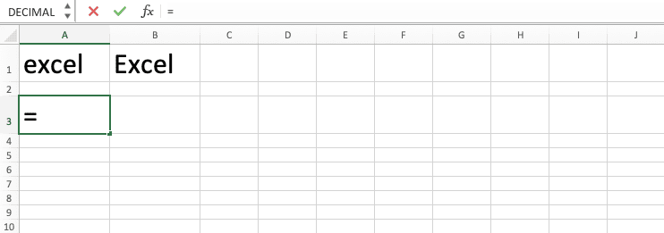
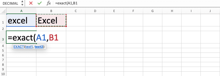
Type an equal sign ( = ) in the cell where you want to put the EXACT result
-
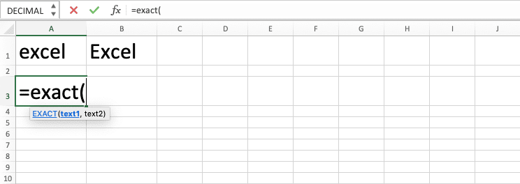
Type EXACT (can be with large and small letters) and an open bracket sign after =
-
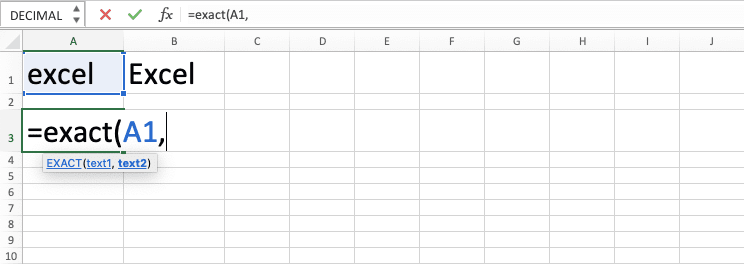
Input the first text you want to compare. Then, type a comma sign ( , )
-
Input the second text you want to compare
-
Type a close bracket sign
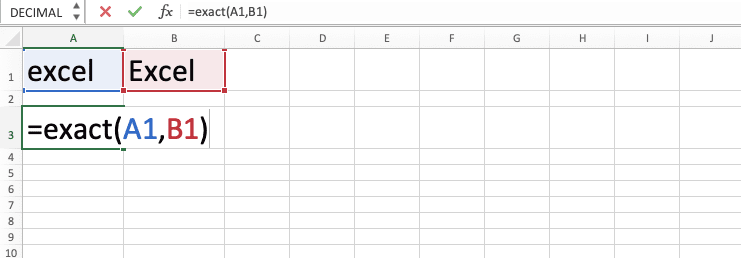
- Type Enter
-
Done!
Count Data in a Cell Range in a Case-Sensitive Manner: SUMPRODUCT EXACT
One of the most useful applications of EXACT is when we combine its writing with SUMPRODUCT. We can use this SUMPRODUCT and EXACT combination to count data in a cell range in a case-sensitive manner.When we have criteria to count data in excel, we usually use COUNTIF or COUNTIFS. However, these two formulas don’t compare the data they count in a case-sensitive manner. Because of this, they will think something like “Apple”, “apple”, or “APPLE” as similar.
To count data with a particular criterion in a case-sensitive manner, we should combine SUMPRODUCT and EXACT instead. Here is the general writing form of these two formulas combination to do that counting process.
= SUMPRODUCT ( — ( EXACT ( criterion , data_range ) )
In this formula writing, we write EXACT inside SUMPRODUCT in brackets with a double minus symbol before the bracket. We input the criterion we want for the counting process and the cell range where we count our data inside EXACT.
Want to learn the process that runs after we combine SUMPRODUCT and EXACT like this? First, let’s see the implementation example of the SUMPRODUCT and EXACT combination in excel.
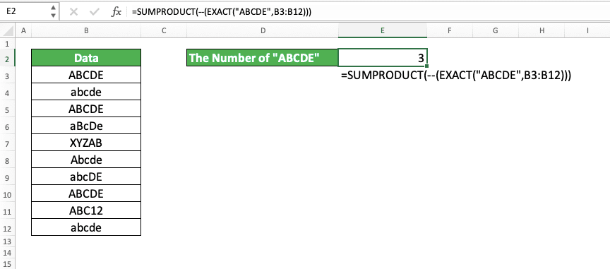
In this example, you can see that we successfully count our data in a case-sensitive manner by using SUMPRODUCT EXACT. We get 3 as the result of SUMPRODUCT EXACT here. That is because there are only 3 data with the same content and letter cases as “ABCDE” in the “Data” column.
How does the SUMPRODUCT EXACT formula writing work so we can get this result? First, because we input data and cell range to EXACT, we will get multiple TRUE and FALSE in an array form. These TRUE and FALSE are results of comparison between the criterion we input (“ABCDE”) with each data in our cell range.
As EXACT is case-sensitive when comparing data, we only get TRUE from data with the same content and letter cases. Thus, this is the TRUE and FALSE array form we get from the EXACT in the example.
{ TRUE , FALSE , TRUE , FALSE , FALSE , FALSE , FALSE , TRUE , FALSE , FALSE }
Notice that we get ten TRUE and FALSE there, the same number as the data amount in the “Data” column. Notice also that the TRUE position corresponds with data similar to “ABCDE”. Meanwhile, the FALSE position corresponds with data not similar to “ABCDE”.
In value, TRUE is the same as 1 and FALSE is the same as 0 in excel. Because of this, we can change the TRUE and FALSE array to a 1 and 0 array using a double minus. That is why we type the symbol in front of the EXACT brackets.
With the help of the double minus, we turn our TRUE and FALSE array into something like this.
{ 1 , 0 , 1 , 0 , 0 , 0 , 0 , 1 , 0 , 0 }
Then, we sum the ones and zeroes in the array with SUMPRODUCT. Usually, we need an array formula form to process an array in excel. But since SUMPRODUCT can process an array too, we don’t need that.
With the sum of the 1 and 0 numbers in the array, we get 3 as our SUMPRODUCT EXACT result. That is the same as the number of “ABCDE” we have in the “Data” column!
Exercise
After you have learned how to use EXACT in excel, now let’s deepen your understanding by doing the following exercise!Download the exercise file and answer the questions. Download the answer key file if you have done the exercise and want to check your answers. Or probably if you are stuck when trying to get the answers for this exercise!
Link to the exercise file:
Download here
Questions
Use EXACT to answer all these questions below in the exercise file!- What is the logic value you get from the comparison between the two texts in row no. 1?
- What is the logic value you get from the comparison between the two texts in row no. 2?
- What is the logic value you get from the comparison between the two texts in row no. 3?
Link to the answer key file:
Download here
Additional Note
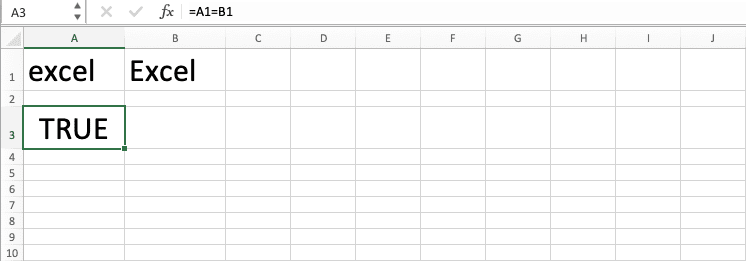
If you don’t have to be case-sensitive when comparing your data, you can just use an equal sign. Place the sign between the two data you want to compare.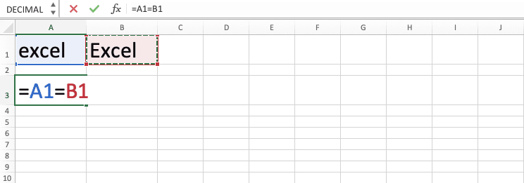
Related tutorials you should learn from: