How to Use Excel RANK Formula: Functions, Examples, and How to Use
Home >> Excel Tutorials from Compute Expert >> Excel Formulas List >> How to Use Excel RANK Formula: Functions, Examples, and How to Use
In this tutorial, you will learn the functions of and how to use the Excel RANK formula completely.
When we work with numbers in excel, we sometimes need to know our number rank in comparison to other numbers. RANK can help you to get that rank easily if you know how to utilize it.
Want to master the RANK formula usage in excel? Read this tutorial until its last part!
Disclaimer: This post may contain affiliate links from which we earn commission from qualifying purchases/actions at no additional cost for you. Learn more
Want to work faster and easier in Excel? Install and use Excel add-ins! Read this article to know the best Excel add-ins to use according to us!
Table of Contents:
- What is the excel RANK formula?
- RANK function in excel
- RANK result
- Excel version from which we can use RANK
- The way to write it and its inputs
- Ranking order in RANK
- Example of its usage and result
- Writing steps
- RANK excel formula application for duplicates (rank them uniquely): RANK COUNTIF
- RANK excel formula application for duplicates (rank them using their average rank): RANK.AVG
- RANK IF in excel (conditional RANK): COUNTIFS
- RANK alternative: RANK.EQ
- Exercise
- Additional note
What is the Excel RANK Formula?
RANK is an excel formula that can help us know a number’s rank when we compare its value to other numbers. The rank can be in a descending or ascending order depending on our preference.RANK Function in Excel
RANK function in excel is to get us the descending or ascending rank of a number in comparison to other numbers.RANK Result
The RANK result is a number that represents the rank of the number we give as its input.Excel Version from Which We Can Use RANK
We can use RANK since excel 2003.The Way to Write It and Its Inputs
Here is the general writing form of the RANK formula in excel.
= RANK ( number , numbers_cell_range , [ order ] )
And here is a bit explanation of the inputs we need to give in our RANK writing.
- number = the number we want to know the rank of in comparison to other numbers
- numbers_cell_range = the cell range containing the numbers we want to compare to the number we inputted earlier. This cell range must also contain the number we want to know the rank of
- [order] = an optional input. Whether we want to know the descending or ascending rank of our number. Input 0 for the descending rank and input 1 for the ascending rank. If we don’t input anything here, then excel will assume our input is 0 (descending rank)
Ranking Order in RANK
In this part, we will discuss a bit further about the third RANK input, the ranking order. This RANK input is important to master if we want to get a correct RANK result.If we want to get the descending rank for our number, then we should input 0 or don’t input anything here. Descending rank is the rank of our number if we order the numbers from largest to smallest. If we want to get a date/time rank, then we get our rank in the newest to oldest order.
If we want to get the ascending rank for our number, then we should input 1 here. Ascending rank is the rank of our number if we order the numbers from smallest to largest. If we want to get a date/time rank, then we get our rank in the oldest to newest order.
Don’t be wrong when giving your ranking order input to RANK. That mistake will most probably make you get a wrong result from your RANK!
Example of Its Usage and Result
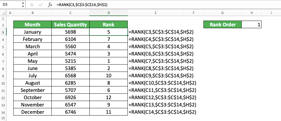
Here is an example of RANK usage and result in excel.
In this example, we want to get the descending and ascending ranks of our monthly sales quantities. We can use RANK if we want to know those ranks quickly.
You can see the writings of the RANK formula to get descending and ascending ranks in the example. If we want to get a descending rank, then we don’t have to input anything for the third RANK input. If we want to get an ascending rank, then we should input 1 for the third RANK input.
For the first RANK input, we input the monthly sales quantity number we want to know the rank of. For the second RANK input, we input the cell range which includes all the monthly sales quantity numbers.
We use dollar symbols in the cell range there because we copy the first RANK writing down to write other RANKs. We don’t want the cell range reference to move when we copy down that first RANK writing (as we should get all our ranks from the comparison with the same group of sales quantity numbers).
Write the RANK formula correctly and we will get the descending/ascending rank we want from our number!
Writing Steps
After we discussed the writing form, inputs, and implementation example of RANK, now let’s discuss its writing steps. In the discussion, there will be an example screenshot for each step so you can understand the RANK writing steps easier.-
Type an equal sign ( = ) in the cell where you want to place your number rank

-
Type RANK (can be with large and small letters) and an open bracket sign after =

-
Input the number you want to get the rank of. Then, type a comma sign ( , )

-
Input the cell range containing your number and the numbers you want to compare it with to get the rank

-
Optional: Type a comma sign. And then, input 0 or 1 to tell RANK whether you want a descending or ascending rank for your number. Input 0 for a descending rank or input 1 for an ascending rank. If you don’t input anything here, you will get a descending rank

-
Type a close bracket sign

- Press Enter
-
Done!
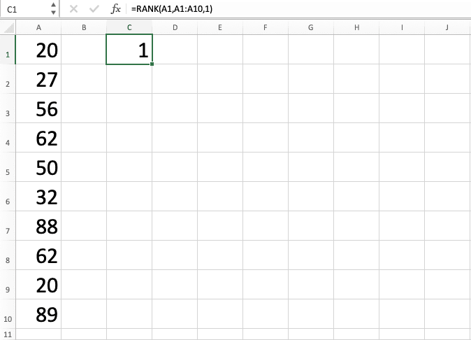
RANK Excel Formula Application for Duplicates (Rank Them Uniquely): RANK COUNTIF
If we have duplicates in our numbers, then we will get the same ranks if we rank them using RANK. That rank will be the highest rank of the duplicates (e.g. if our duplicates rank 6 and 7, then RANK will rank them 6 and 6).What if we want unique ranks for each of our duplicates instead? We can combine RANK and COUNTIF in one formula writing to do that!
Here is the general formula writing form of the RANK and COUNTIF combination to give unique ranks for our duplicate numbers.
= RANK ( number , numbers_cell_range , [ order ] ) + COUNTIF ( parallel_numbers_cell_range_with_number , number ) - 1
The numbers cell range we give to RANK and COUNTIF here is a bit different. The RANK numbers cell range will include all numbers we want to compare in our ranking process from the start. Meanwhile, the COUNTIF numbers cell range will only include numbers until the cell that contains our number.
The RANK in the formula writing there will work as usual. When there is no duplicate for our number in the numbers cell range, we will definitely get 1 from our COUNTIF. That is because the counting criterion we use is our number and we count its occurrence in our numbers cell range.
However, since we add -1 in the formula writing, it will cancel out the 1 we get from our COUNTIF. Thus, if the number we rank isn’t a duplicate, then we will get our RANK result only.
However, when our number is a duplicate, our COUNTIF result should become more than 1. It keeps adding up if there are already duplicates before in our numbers cell range. As we add our RANK result with the COUNTIF result, we will get a unique rank for each of our duplicates!
For a better understanding of the formula concept, here is its implementation example in excel.

In this example, we want to get the rank of the regions based on the number of branches they have. We use RANK only and RANK plus COUNTIF to get our ranks to compare their results.
As you can see, RANK and COUNTIF produce different results when they rank duplicate numbers. RANK will give them the same rank while RANK and COUNTIF will give them a unique rank. For unique numbers, the results of RANK and COUNTIF and RANK only are the same.
The mechanism why RANK with COUNTIF can give unique ranks is as we have discussed previously. COUNTIF result will add to our RANK result as we find more duplicates for a particular number. Meanwhile, -1 in the RANK and COUNTIF formula writing will make us get the correct ranks.
As for the dollar symbols in the RANK and COUNTIF cell range inputs, we use them for our formula copy process. This is so the cell range inputs won’t move when we copy down our first formula writing to get all ranks.
For COUNTIF, we put dollar symbols only in the first cell of the cell range. This is so the second cell can still follow our copy process. Remember, we only want the numbers from the first cell until the cell that contains our number in it.
RANK Excel Formula Application for Duplicates (Rank Them Using Their Average Rank): RANK.AVG
What if we want to rank our duplicate numbers with an average rank instead? For example, if our duplicates rank 6 and 7, then we want their ranks to become 6.5 and 6.5.We can have this kind of rank easily if we use RANK.AVG formula instead of RANK. You can use the RANK.AVG formula if you have excel version 2010 onwards.
The general writing form of RANK.AVG is almost similar to RANK as you can see below.
= RANK.AVG ( number , numbers_cell_range , [ order ] )
The rank we get from RANK.AVG is almost similar to RANK. The only difference between them is the rank we get if we rank duplicates. RANK.AVG will give us the duplicates’ average rank while RANK will give us the highest rank of the duplicates.
You can see the implementation example of RANK.AVG and its clear comparison with RANK below.

As you can see there, we get the same results from RANK.AVG and RANK except for numbers that have duplicates. RANK.AVG ranks 6 for 15 branches (the average of 5, 6, and 7) and 14.5 for 5 branches (the average of 14 and 15). On the other hand, RANK ranks 5 for 15 branches and 14 for 5 branches.
Whenever you need an average rank for your duplicate numbers, use RANK.AVG instead of RANK!
RANK IF in Excel (Conditional RANK): COUNTIFS
Want to rank your number in comparison to other numbers that have the same criteria?Unfortunately, Excel doesn’t provide us with formulas like RANKIF or RANKIFS to do that kind of ranking. However, there is an alternative method we can implement to do a conditional ranking process like that in excel. This method utilizes COUNTIFS for its purpose.
The general writing form of COUNTIFS so it can work as an alternative RANK IF formula is as follows.
= COUNTIFS ( data_range1 , criterion1 , … , numbers_range1 , “>” & number ) + 1
We input the cell ranges we want to evaluate with our criteria and the criteria themselves to COUNTIFS. We also input our numbers cell range and the number which rank we want to know in the formula.
As usual, when using COUNTIFS, the cell range and the criterion/number inputs must be in pairs. The criterion we input will only evaluate the data in the cell range we input just before it.
We need to input a “>” or “<“ with the “&” symbol too when we input our number in COUNTIFS. This is so we can get the rank result we want from our COUNTIFS.
Use “>” if you want to get a descending rank and use “<“ if you want to get an ascending rank. The number of numbers that are more than or less than our number will help to give us our rank result. The “&” symbol there will help join the “>”/“<“ symbol with our number input.
We use COUNTIFS here because we want to rank our number in comparison to other numbers with similar criteria. Therefore, we should use our number criteria as the COUNTIFS criteria inputs.
COUNTIFS will only count the data entries that fulfill all their corresponding criteria. This will help us rank our number with the comparison only to other numbers that have similar characteristics as it has!
Moreover, we also add “+1” in our COUNTIFS formula writing there. This is so we can get the correct conditional rank result from our COUNTIFS.
To better understand how COUNTIFS can help us rank our number, here is its implementation example in excel.
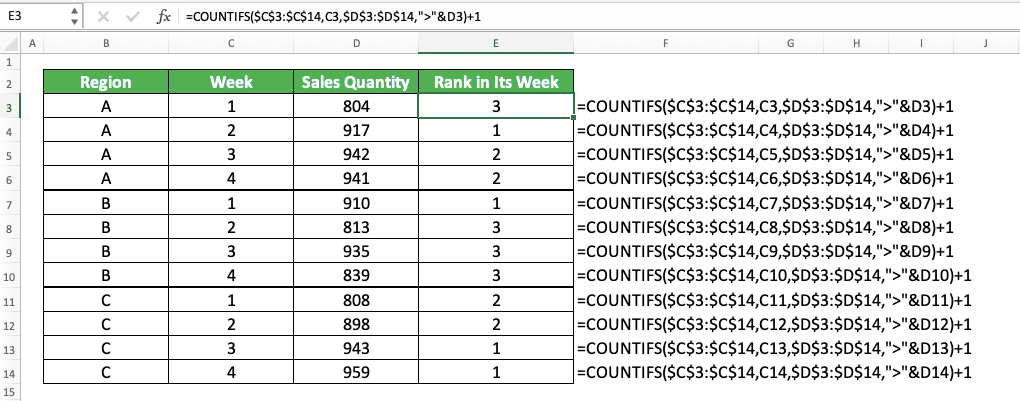
In the example, we want to rank our sales quantities in comparison with other sales quantities in their week. As we have a week criterion for our ranking process, we use COUNTIFS to help us get our ranks.
We input the week cell range and the week of the number we want to rank with our COUNTIFS here. We also input the sales quantity numbers cell range and the sales quantity we want to know the rank of. We use the “>” symbol here because we want to get the descending rank of our sales quantity.
COUNTIFS will make us process only the sales quantities in the same week as the sales quantity we want to rank. As we use “>” in the sales quantity criterion, we will only count the sales quantities with more values. This is similar to getting the descending rank of our sales quantity as we also add 1 to the result.
We write our COUNTIFS according to what we have discussed. As a result, we will get the rank of our number in comparison to other numbers in its group!
RANK Alternative: RANK.EQ
If you use excel 2010 onwards, then you can use RANK.EQ as an alternative to RANK. The function, writing, and result of RANK.EQ is similar to RANK.The general writing form of RANK.EQ in excel is as you can see below.
= RANK.EQ ( number , numbers_cell_range , [ order ] )
Quite similar to RANK, isn’t it? And here is the RANK.EQ implementation example in excel. You can see the comparison of the results we get from RANK.EQ and RANK here.
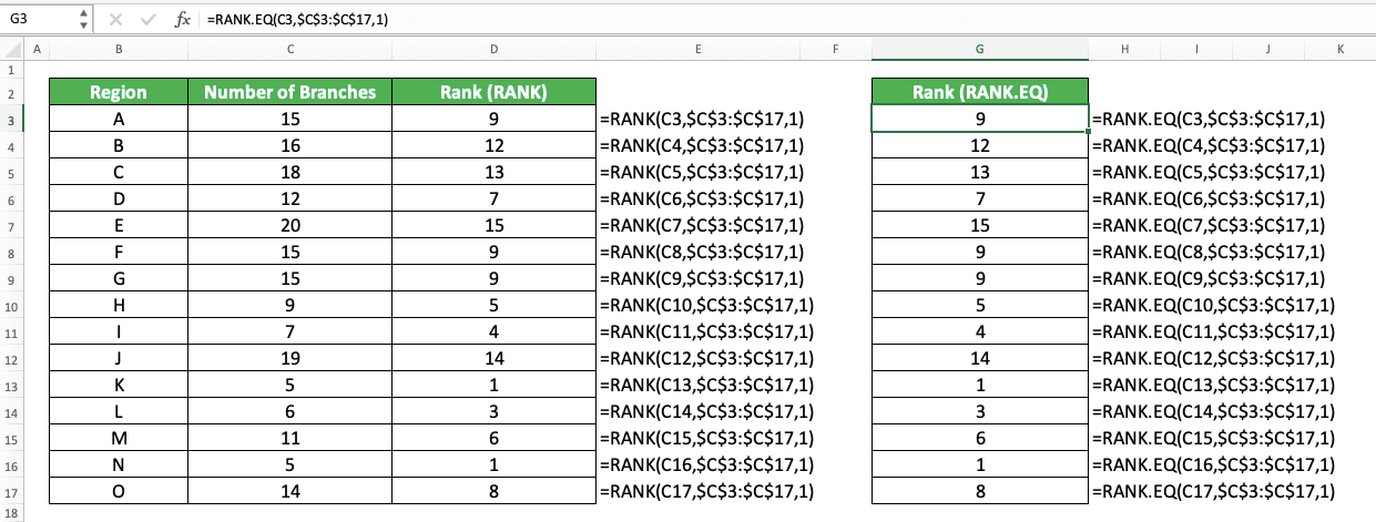
As you can see there, we get the same results from RANK.EQ and RANK when we rank our numbers. We also get the highest possible rank for our duplicate numbers when we use either formula.
If you need an alternative formula to RANK, consider using the RANK.EQ formula!
Exercise
After learning how to use the RANK formula in excel completely, now let’s do an exercise. This is so you can understand more about the implementation of RANK in excel.Download the exercise file from the following link and answer the questions below. Download the answer key file if you have finished the exercise and want to check your answers.
Link to the exercise file:
Download here
Questions
- What is the descending rank of 387 in column B?
- What is the ascending rank of 717 in column C?
- What is the ascending rank of 484 in comparison to the numbers in all columns?
Link to the answer key file:
Download here
Additional Note
To toggle between descending and ascending rank of your number easily, input a cell coordinate for your RANK’s ranking order. That way, you just need to alternate between 0 (or just delete the cell value) and 1 in your cell to toggle your number’s rank!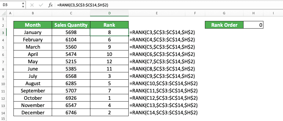
Related tutorials you should learn:


