How to Rank in Excel with Various Excel Ranking Formulas
Home >> Excel Tutorials from Compute Expert >> Excel Calculations >> How to Rank in Excel with Various Excel Ranking Formulas
In this tutorial, you will learn how to rank in excel with various excel ranking formulas.
When working with numbers in excel, we sometimes need to know the rank of some numbers in comparison to other numbers. To get those ranks correctly, you should understand how to rank in excel with the right methods. There are some formulas and features you can use to help you with your ranking process.
Want to know what are those formulas and features and how to rank in excel in various situations? Read this tutorial until its last part!
Disclaimer: This post may contain affiliate links from which we earn commission from qualifying purchases/actions at no additional cost for you. Learn more
Want to work faster and easier in Excel? Install and use Excel add-ins! Read this article to know the best Excel add-ins to use according to us!
Table of Contents:
- How to rank in excel normally
- How to rank data in excel with the sorting process
- How to rank duplicates in excel without skipping ranks after that
- How to rank in excel with an average rank for duplicates
- How to rank duplicates uniquely in excel
- How to rank in excel conditionally/based on multiple criteria (RANK IF)
- How to get a percentile rank in excel
- How to rank in excel by ignoring zeroes
- How to rank positive and negative numbers separately
- How to rank in excel using absolute values
- How to rank in non-adjacent cells
- How to rank in excel by group
- How to do weighted ranking in excel
- How to do dynamic ranking in excel
- How to rank in a pivot table
- How to get nth largest/smallest values in excel
- Exercise
- Additional note
How to Rank in Excel Normally
Excel provides us with special formulas that we can use to rank our numbers in it. Those formulas are RANK and RANK.EQ.These two formulas have the same usefulness and the way to write them is also similar. RANK.EQ is officially an updated version of RANK (we can use it since excel 2010) although there seems to be nothing that separates these two.
To use RANK and RANK.EQ, you can write them in this kind of form.
RANK
= RANK ( number_to_rank , numbers_cell_range , [ order ] )
RANK.EQ
= RANK.EQ ( number_to_rank , numbers_cell_range , [ order ] )
Not much difference, right? You need to input the number to rank and the cell range containing numbers you want to compare for the rank (the cell range should include the number you want to rank too).
If you need to, then you should also input whether you want to rank in descending or ascending order. Input 0 for descending and input 1 for ascending. If you don’t input anything, then excel will assume you want a descending order rank.
Use RANK or RANK.EQ and you should get the same result! You can see their implementation example in excel in the following screenshot.
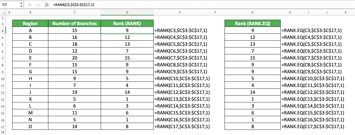
In the example, we try to rank the regions there according to the number of branches they have. We use RANK and RANK.EQ to help with the ranking process.
As you can see, we write RANKs and RANK.EQs we need with the writing form we have discussed before. We input the region’s number of branch we want to rank and the number of branches column cell range. As we want to get ascending ranks here, we input 1 for the order input of our RANK and RANK.EQ.
As a result, we get the same ranks from the RANKs and RANK.EQs we write!
How to Rank Data in Excel with the Sorting Process
If you want to rank your numbers while placing them in their ranking order too, utilize the sorting feature in excel. After you sort your numbers, you should be able to tell their rank easily by seeing their position.You can sort your numbers in the order you want, whether it is descending or ascending. The way to do it is also quite simple as you can see in the step-by-step below.
-
Highlight the column cell range containing the numbers you want to sort

-
Go to the Data tab and click either the Sort Smallest to Largest (ascending) or Sort Largest to Smallest (descending) button there. Choose the button according to in what order you want to see your numbers rank

-
In the dialog box that shows up, there are two sorting options you can choose. Choose “Expand the selection” if you want to sort adjacent columns too with the sorting basis from your numbers column. Choose “Continue with the current selection” if you want to only sort the numbers column you currently highlight.
Click the Sort button after you choose the option you want

-
Done! You have sorted your numbers column! Now, you should be able to see your numbers rank in the order you want easily

How to Rank Duplicates in Excel Without Skipping Ranks After That
You can see in their implementation example earlier that we skip if after we rank duplicates using RANK and RANK.EQ. For example, if we rank 3, 3, and 5 numbers, then the 5 there will get rank 3. That is because RANK and RANK.EQ count the number of duplicates too to rank the next number after them.What if in the case of 3, 3, and 5, we want to rank the 5 there with 2, not 3? How we can make it so excel doesn’t skip ranks after it ranks the duplicates we have?
One of the methods we can utilize is to combine SUMPRODUCT and COUNTIF to rank our numbers.
Here is the general writing form of the SUMPRODUCT and COUNTIF in excel to rank numbers without skipping ranks.
= SUMPRODUCT ( ( number_to_rank <= numbers_cell_range ) / COUNTIF ( numbers_cell_range , numbers_cell_range ) )
This formula writing assumes that we want to rank our number in descending order. If we want to rank our number in ascending order, replace the <= symbol with >=.
Want to learn more about the logic behind the formula writing? We will discuss it through its implementation example below so you can understand easier!
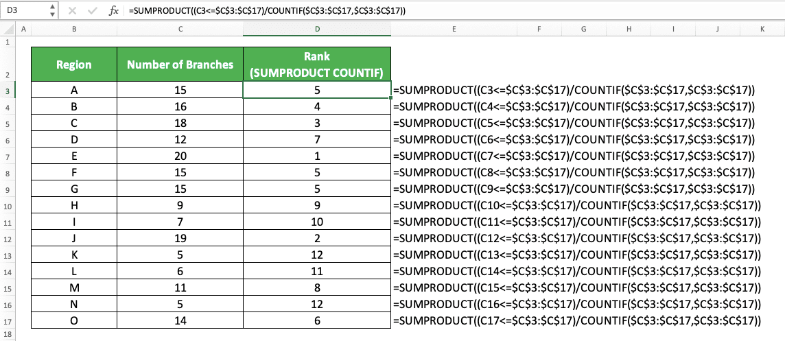
Here, we use the same data set we use in the RANK and RANK.EQ implementation example earlier. As you can see, by combining SUMPRODUCT and COUNTIF, we can make excel not skipping ranks after it ranks duplicate numbers.
What is the logic behind the formula writing so we can get the ranking results we want? First, let’s take a look at the first half of our SUMPRODUCT input before the COUNTIF.
There, we input (number_to_rank<=numbers_cell_range). We input something like this because we want to filter numbers that are less than or equal to our number. As we calculate descending ranks in the example, we get our number rank by filtering like this first.
As we compare our number with a cell range, we will get a TRUE/FALSE array result from the operation. We get TRUE if the number in the cell range is more than or equal to our number. We get FALSE if the number in the cell range is less than our number.
In the example, we get a TRUE/FALSE array like this from the input of region A with 15 branches.
{ TRUE , TRUE , TRUE , FALSE , TRUE , TRUE , TRUE , FALSE , FALSE , TRUE , FALSE , FALSE , FALSE , FALSE , FALSE }
We will divide this array with the COUNTIF result.
In our COUNTIF, we input our numbers cell range twice. This is because we want to get an array containing the number of each number in the numbers cell range. The COUNTIF cell range input is our numbers cell range and the counting criterion is each number in the cell range.
From the COUNTIF we write in the example, we get an array like this for each region.
{ 3 , 1 , 1 , 1 , 1 , 3 , 3 , 1 , 1 , 1 , 2 , 1 , 1 , 2 , 1 }
The result is the same for each region because we input the same number cell ranges in our COUNTIF.
As we get our two arrays, we divide them by using the slash symbol we write between them in our formula. We can divide the TRUE/FALSE because TRUE is the same as 1 and FALSE is 0 in excel.
As an array division process divides numbers in similar array positions, we get this result for region A in the example.
{ 0.333 , 1 , 1 , 0 , 1 , 0.333 , 0.333 , 0 , 0 , 1 , 0 , 0 , 0 , 0 , 0 }
We sum all the numbers in the array division result using SUMPRODUCT. We use SUMPRODUCT because it can help us to process arrays too without having to use an array formula form.
For region A in the example, we get 5 after we sum the array division result. That is the rank of the number of branches in comparison to other regions’ number of branches! As we get decimals for the numbers which have duplicates, we don’t need to skip ranks after ranking our duplicates.
As an additional note, you may notice we use dollar symbols in the example formula writing. That is because we copy down our first formula writing to get all the formula writings we need there.
Using dollar symbols makes the numbers cell range input doesn’t move and this is what we need. After all, we use the same numbers cell range input in all our formula writings there.
How to Rank in Excel with an Average Rank for Duplicates
What if we are okay with skipping ranks but we want to rank the duplicates with an average rank? That means if we rank 3 in a 3 , 3 , 5 group, the rank will be 1.5 (the average of rank 1 and 2 for the two 3s) instead of 1 (the highest rank between rank 1 and 2 for the two 3s).If you want something like that, then you can use RANK.AVG to get average ranks for duplicates. The general writing form of RANK.AVG in excel is similar to RANK and RANK.EQ.
= RANK.AVG ( number_to_rank , numbers_cell_range , [ order ] )
And here is its implementation example in excel. As you can see here, RANK.AVG ranks duplicates in their average rank instead of their highest possible rank.
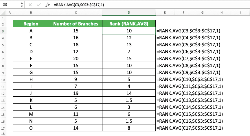
When you need to rank your duplicates with an average rank, use RANK.AVG!
How to Rank Duplicates Uniquely in Excel
From all the formula methods we have used to rank our duplicate numbers, we get the same ranks. What if we want to rank them uniquely so all our numbers can get a unique rank? We can combine RANK and COUNTIF to do the unique ranking process.The way to write the RANK and COUNTIF combination for the unique rank purpose is as follows.
= RANK ( number_to_rank , numbers_cell_range , [ order ] ) + COUNTIF ( parallel_numbers_cell_range_with_number_to_rank , number_to_rank ) - 1
We write our RANK formula normally there while adding a COUNTIF result and subtract the addition result with one.
In the COUNTIF, we input our numbers cell range from the first number until the cell containing the number to rank. This is so we can rank our duplicates uniquely according to the number of times they have appeared. We put minus one there too to adjust the result so we can get the right rank for our numbers.
The implementation example of this RANK and COUNTIF combination in excel is as follows.

As you can see there, we get unique ranks for each duplicate we have in our numbers (15 and 9). This is because we combine RANK and COUNTIF to get our ranks.
In the COUNTIF, we input our numbers cell range by using dollar symbols in its first cell coordinate. The first cell coordinate is the cell containing the first number and the second is the parallel cell with our number.
The dollar symbols cause the COUNTIF cell range input to follow when we copy our formula writing. Thus, we can get the correct cell range input for each of our COUNTIFs!
We write our RANK and COUNTIF combination according to the writing form we have discussed. As a result, we get the rank for all our numbers uniquely!
How to Rank in Excel Conditionally/Based on Multiple Criteria (RANK IF)
We may have some characteristics in the number we want to rank. Sometimes, we probably want to rank the number only in comparison to the numbers that have the same characteristics.Unfortunately, we don’t have a formula like RANKIF or RANKIFS to help us rank like that. However, we can use COUNTIFS as an alternative to doing that kind of ranking process.
Here is the COUNTIFS general writing form to help us rank conditionally.
= COUNTIFS ( data_range1 , criterion1 , … , numbers_range , “>” & number_to_rank ) + 1
As ever, we input the cell ranges and criteria to our COUNTIFS in pairs. The criterion we input will only evaluate the data in the cell range we input before it.
To rank a number in comparison to the numbers with the same characteristics, input the number characteristics as the criteria. We pair a relevant cell range with each of our number characteristics so we can get the right rank result.
We also input the cell range containing our numbers and the comparison to the number we rank as the criterion. For the comparison, we write “>” if we want a descending rank and “<“ if we want an ascending rank. We write an ampersand (&) too to connect the symbol with our number.
Logically, the fewer numbers that are more than the number we want to rank, the higher descending rank we should get. The fewer numbers that are less than the number we want to rank, the higher ascending rank we should get too.
The comparison criterion makes us count our numbers correctly and get our rank based on the counting result. We add plus one too in our formula writing so we can adjust our COUNTIFS result to get the correct rank.
For a better understanding of the COUNTIFS concept, here is an implementation example of it in excel.
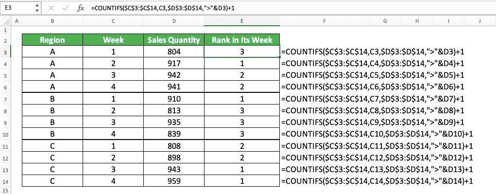
In the example, we want to rank our sales quantities in their week group. That means we only want to compare with the sales quantities in the same week to get our rank.
We use COUNTIFS to help us do the ranking process. As the week is our criterion here, we input the week column cell range and the sales quantity week to COUNTIFS.
We also input the sales quantity column cell range and its comparison with the sales quantity as the criterion. As we want descending ranks here, we input “>” as the comparison symbol.
We do all that and we get our sales quantities ranks in comparison to other sales quantities in the same week!
How to Get a Percentile Rank in Excel
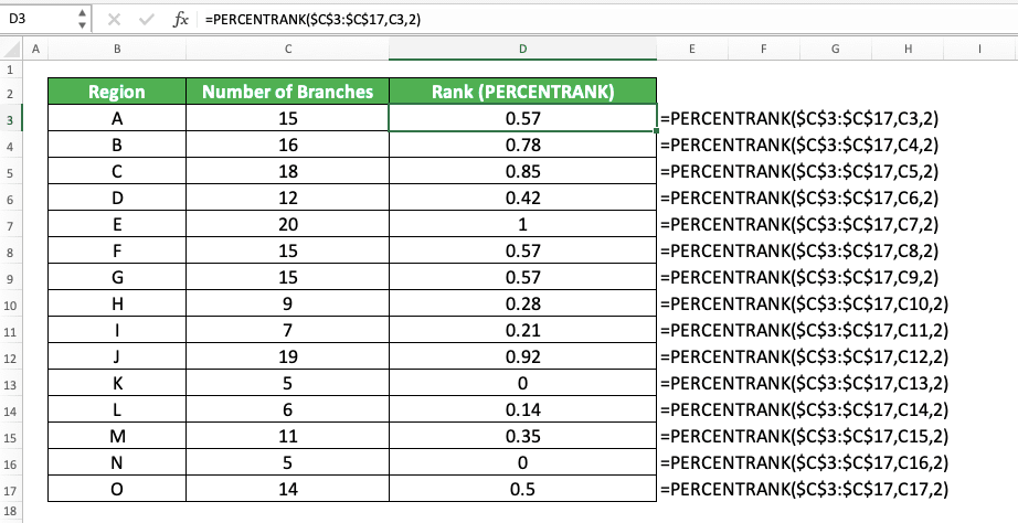
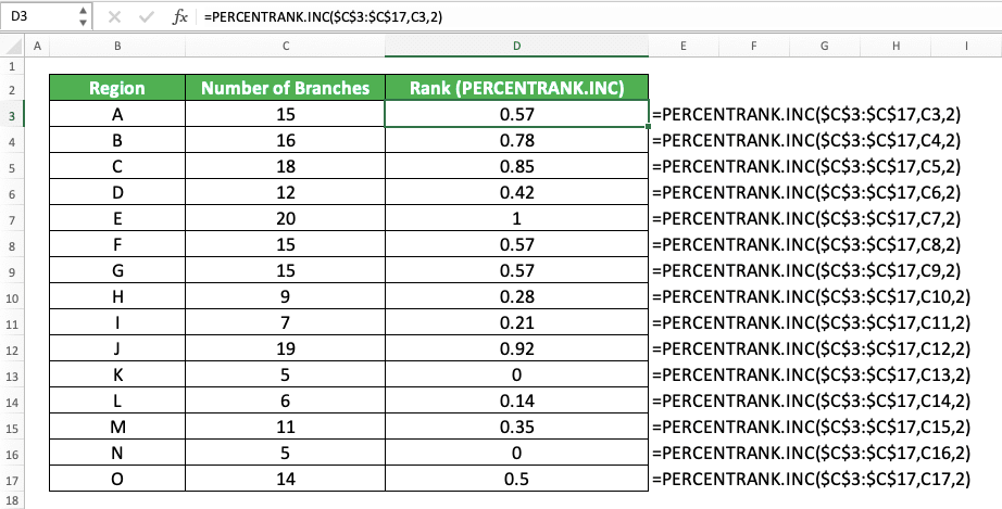
Need to get your number rank in the form of percentile in comparison to other numbers? You can use PERCENTRANK/PERCENTRANK.INC/PERCENTRANK.EXC to help you.The percentile ranking is the rank of your number in comparison to other numbers in terms of percentage. The scale of the ranking is from 0 to 1. For example, if your number is larger than 30% of other numbers, it will get a 0.3 percentile rank.
PERCENTRANK/PERCENTRANK.INC/PERCENTRANK.EXC can get you the percentile rank of your numbers in excel. PERCENTRANK.EXC and PERCENTRANK.INC are the newer versions of PERCENTRANK officially that you can use since excel 2010. However, you can still use PERCENTRANK if you want to.
Use PERCENTRANK.EXC to be exclusive with the first and the last number in your numbers for the percentile ranking. Use PERCENTRANK or PERCENTRANK.INC if you want to be inclusive with those numbers instead.
Here is the general writing form of these three formulas in excel.
= PERCENTRANK/PERCENTRANK.INC/PERCENTRANK.EXC ( numbers_cell_range , number_to_rank , [ significance ] )
The three formulas require the same inputs in their writing. The significance input there is the number of decimals you want for your percentile rank result. If you don’t input anything for the significance, then excel assumes you want the significance of three.
To better understand these formulas, here are their implementation examples in excel.
PERCENTRANK
PERCENTRANK.INC
PERCENTRANK.EXC
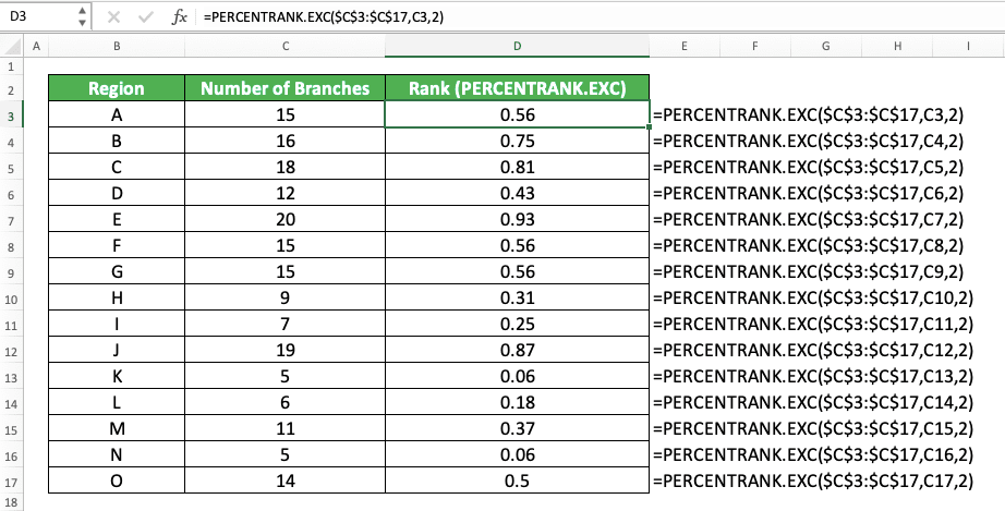
As you can see in the examples, we get different percentile ranks from PERCENTRANK.EXC and PERCENTRANK/PERCENTRANK.INC. That is because of the exclusive and inclusive nature in each of those three formulas.
Use the correct formula, either PERCENTRANK, PERCENTRANK.INC, or PERCENTRANK.EXC according to your percentile rank calculation needs!
How to Rank in Excel by Ignoring Zeroes
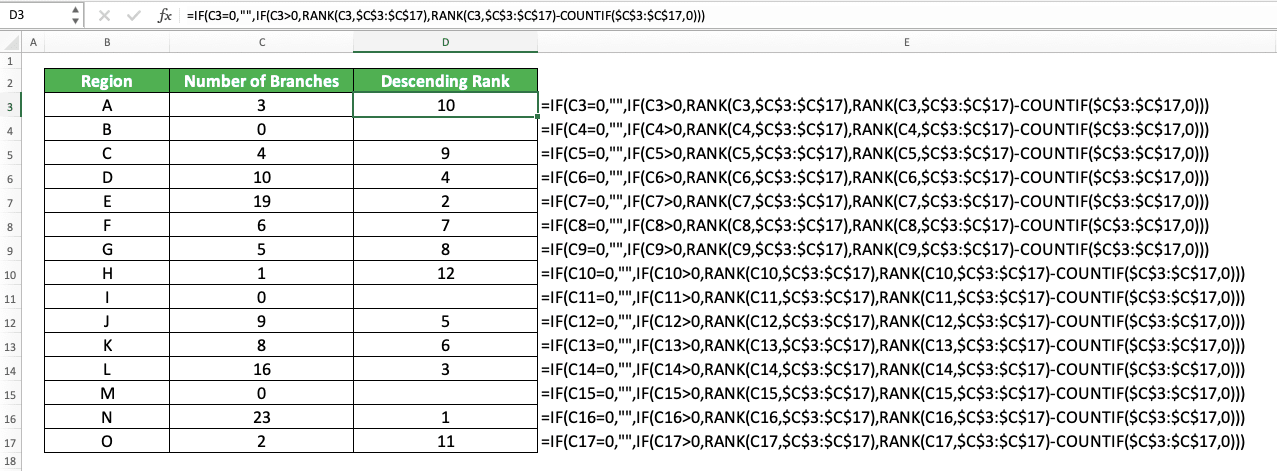
Sometimes, we have zeroes in our numbers and we want to ignore them in our ranking process. To do that in excel, we can combine IF, RANK, and COUNTIF to help us get the ranks.Here are the general writing forms of the IF, RANK, and COUNTIF combination to ignore zeroes in our ranking process. We have a different writing form to rank in descending order and to rank in ascending order.
Rank in descending order
= IF ( number_to_rank = 0 , “” , IF ( number_to_rank > 0 , RANK ( number_to_rank , numbers_cell_range ) , RANK ( number_to_rank , numbers_cell_range ) - COUNTIF ( numbers_cell_range , 0 ) ) )
Rank in ascending order
= IF ( number_to_rank = 0 , “” , IF ( number_to_rank > 0 , RANK ( number_to_rank , numbers_cell_range , 1 ) - COUNTIF ( numbers_cell_range , 0 ) , RANK ( number_to_rank , numbers_cell_range , 1 ) ) )
As we want to ignore zeroes, we make our IF produce blank if we find zeroes in our numbers. In the IF, we use COUNTIF to adjust our rank results from RANK correctly so zeroes don’t affect them. The COUNTIF counts the number of zeroes we have in our numbers cell range.
If we rank in descending order, then we input our COUNTIF if we rank negative numbers. If we rank in ascending order, then we input our COUNTIF if we rank positive numbers. We do this because zeroes affect the negative and positive numbers ranking process in different ranking orders.
Here are the implementation examples of the IF, RANK, and COUNTIF combination in excel. We separate the process to rank in descending and ascending order in a different example.
Descending order example
Ascending order example
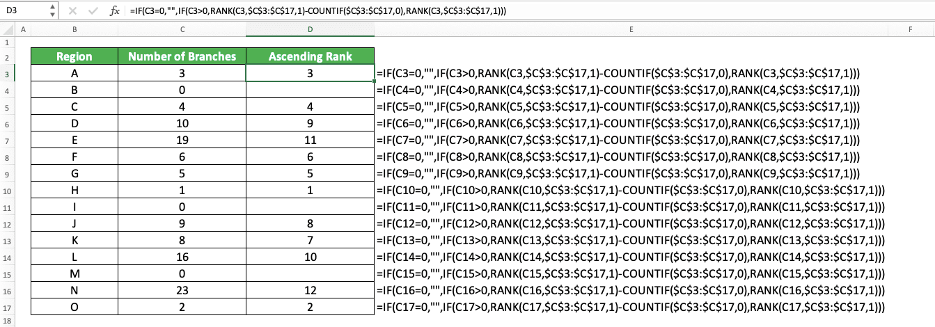
As you can see in the examples, we successfully ignore zeroes in our ranking process! That is because we write our IF, RANK, and COUNTIF combination correctly.
For the descending order ranks, we write our COUNTIF in the negative numbers ranking process part in our IF. And for the ascending order ranks, we write our COUNTIF in the positive numbers ranking process part in our IF. We write our RANK formula normally in both ranking orders.
How to Rank Positive and Negative Numbers Separately
Need to rank your positive/negative numbers in comparison to other positive/negative numbers only? As this looks like some kind of criterion for your ranking process, you can use COUNTIFS to help you. Combine it with IF to get a blank if the number isn’t the positive/negative number you want to rank.The way to combine IF and COUNTIFS to rank your positive/negative numbers in descending/ascending order is as follows.
Rank positive numbers in descending order
= IF ( number_to_rank > 0 , COUNTIFS ( numbers_cell_range , “>” & number_to_rank ) + 1 , “” )
Rank positive numbers in ascending order
= IF ( number_to_rank > 0 , COUNTIFS ( numbers_cell_range , “<“ & number_to_rank , numbers_cell_range , “>0” ) + 1 , “” )
Rank negative numbers in descending order
= IF ( number_to_rank < 0 , COUNTIFS ( numbers_cell_range , “>” & number_to_rank , numbers_cell_range , “<0” ) + 1 , “” )
Rank negative numbers in ascending order
= IF ( number_to_rank < 0 , COUNTIFS ( numbers_cell_range , “<“ & number_to_rank ) + 1 , “” )
We put our COUNTIFS in our IF and make it its TRUE result. For the IF logic condition, we put the positive/negative number condition.
In the COUNTIFS, we put a criterion for the numbers in our cell range depending on the ranking order we want. If we want a descending order rank, we input the criterion of more than (“>”) the number we want to rank. If we want an ascending order rank, we input the opposite criterion (“<“).
If we rank positive numbers in ascending order, we need to input a positive number criterion in our COUNTIFS. That is because it is possible for the number less than the number we want to rank to be negative. We do the same thing too if we rank negative numbers in descending order for a similar reason.
We also add one there to our COUNTIFS result so we can get the correct rank for our positive/negative number.
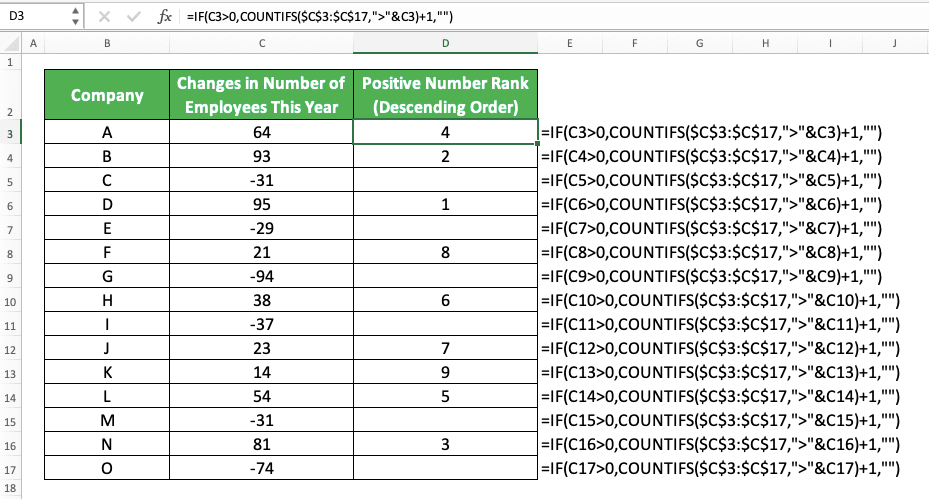
For a better understanding of the IF and COUNTIFS combination concept, here are its implementation examples in excel.
Rank positive numbers
Rank negative numbers
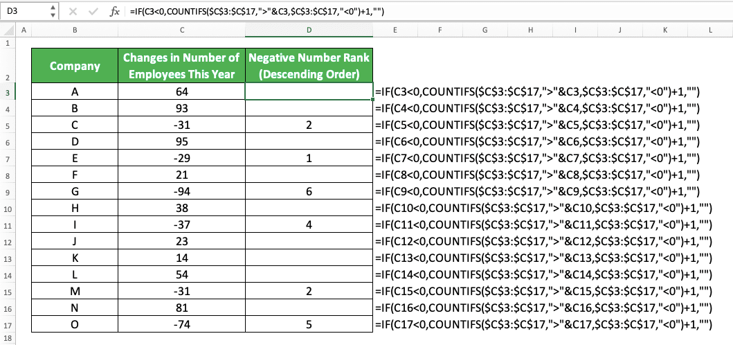
In the examples, we rank our positive and negative numbers in descending order. We can rank each of them separately using the IF and COUNTIFS combination as you can see there.
When we want to rank positive numbers only, we ignore the negative numbers in our ranking process completely. The opposite is also true. When we want to rank negative numbers only, we ignore the positive numbers completely.
We write the IF and COUNTIFS combination in the examples using the writing form we have discussed just now. As a result, we get the positive and negative numbers ranking results we need correctly!
How to Rank in Excel Using Absolute Values
Instead of ranking our positive and negative numbers separately, we may want to rank their absolute values together instead. That means we just compare the number values in our ranking process without looking at the positive or negative number symbol.Is there a way to do this kind of ranking process in excel? Yes, there is. We can combine SUMPRODUCT and ABS to rank our numbers’ absolute values fast!
Here is the general writing form of the SUMPRODUCT and ABS combination for the purpose.
Ranking absolute values in descending order
= SUMPRODUCT ( — ( ABS ( number_to_rank ) < ABS ( numbers_cell_range ) ) ) + 1
Ranking absolute values in ascending order
= SUMPRODUCT ( — ( ABS ( number_to_rank ) > ABS ( numbers_cell_range ) ) ) + 1
In the formula writing, we implement ABS to our number and numbers cell range in SUMPRODUCT. We use ABS to get the absolute values of the number we want to rank and numbers in our cell range.
We compare the number we want to rank with each number we have in our cell range in their absolute values. The comparison symbol we use depends on the order we want for our rank. We use the “<“ symbol for a descending rank and “>” for an ascending rank.
We get a TRUE/FALSE array result as the result of the comparison of the numbers. We use the double minus symbol in front of the ABS writing there to turn the TRUE/FALSE to 1/0.
Then, we use SUMPRODUCT to sum the ones and zeroes in the array and add one to the sum result. From there, we get our number absolute value rank in the order that we want!
The implementation example of this SUMPRODUCT and ABS combination is as follows.
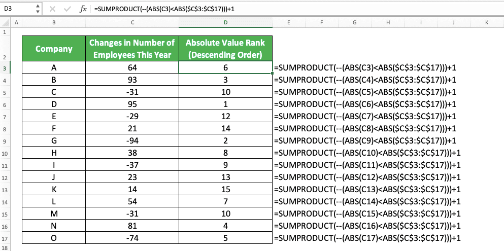
As you can see, by using the SUMPRODUCT and ABS combination, we can get the ranks of our numbers absolute values!
How to Rank in Non-Adjacent Cells
Need to rank numbers in non-adjacent cells? To do it smoothly, you need to combine IF, ISNA, and RANK in your formula writing for the ranking process. When inputting the RANK, you need to input just the non-adjacent cells, not the whole numbers cell range.Here is the general writing form of the IF, ISNA, and RANK combination to rank in non-adjacent cells.
= IF ( ISNA ( RANK ( number_to_rank , ( non-adjacent_cells ) , [ order ] ) ) , “” , RANK ( number_to_rank , ( non-adjacent_cells ) , [ order ] ) )
We write our RANK in our IF twice here, as the ISNA input and as the IF FALSE result. We write it normally except for the non-adjacent cells in brackets that replace our usual numbers cell range.
We use IF and ISNA here to anticipate #N/A errors. When we copy the formula writing, the cells that we don’t include in our ranking process will produce #N/A. So, to make the cells display better, we change the #N/A errors to blank instead here.
To better understand the concept, here is its implementation example in excel.

In the example, we try to rank the number of branches in five regions (B, E, H, K, and O) from the fifteen we have there. As the five regions’ number of branches are in non-adjacent cells, we rank using the IF, ISNA, and RANK combination.
We write the RANK by inputting the number to rank and the non-adjacent cells for the numbers cell range. We put it inside ISNA and as the FALSE result of our IF. When ISNA produces TRUE (which means we get a #N/A error), we want our IF to produce blank.
We do that and we get our ranks in non-adjacent cells as you can see in the example!
How to Rank in Excel by Group
Want to rank your numbers according to the numbers in the same group? As we usually define a data group by its data similar characteristics, we can use COUNTIFS to help us rank here.The way to use the COUNTIFS is the same as the way we use it to rank conditionally before. Input the data cell range where the group characteristic is and the characteristic itself in pairs to the COUNTIFS. Input until you have inputted all of the characteristics that define your data groups.
Moreover, input your number cell range and the number criterion also. Input the “>” symbol in the number criterion if you want descending ranks. If you want ascending ranks, input the “<“ symbol.
Do it correctly as we have discussed previously about ranking conditionally using COUNTIFS. You will get your number ranks in comparison to the numbers in the same group!
How to Do Weighted Ranking in Excel
Weighted ranking means that you rank your numbers relative to the rank of the smallest and largest number. If a number is nearer to the largest number, then the number rank should be nearer to the largest number rank. The opposite is also true.We don’t have a special formula to do a weighted ranking calculation process in excel. Thus, we must create the formula manually using RANK and also MAX and MIN to get the largest and smallest numbers. We need them as the comparison for other numbers we want to rank.
The formula writing that incorporates RANK, MAX, and MIN formulas is as follows. We separate the writing for descending and ascending rank here.
Weighted ranking (descending order)
= 1 + ( MAX ( numbers_cell_range ) - number_to_rank ) / ( MAX ( numbers_cell_range ) - MIN ( numbers_cell_range ) ) * ( RANK ( MIN ( numbers_cell_range ) , numbers_cell_range ) - 1 )
Weighted ranking (ascending order)
= 1 + ( number_to_rank - MIN ( numbers_cell_range ) ) / ( MAX ( numbers_cell_range ) - MIN ( numbers_cell_range ) ) * ( RANK ( MAX ( numbers_cell_range ) , numbers_cell_range , 1 ) - 1 )
Those formula writings look complicated but the concept behind them is actually quite simple. In each writing, we try to compare between the number we want to rank and the largest and smallest numbers.
For descending ranks, we get the difference between our number and the largest number. Then, we divide it with the difference between the largest number and the smallest number.
After we get the difference comparison, we multiply it with the descending rank of the smallest number (the largest rank). We adjust the result by adding and subtracting it with one to get the correct weighted rank. For the ascending ranks, we do similar things with a bit of adjustment on the formula ranking process.
For a better understanding of the weighted ranking formula writings, you can see their implementation examples below.
Weighted ranking (descending order)

Weighted ranking (ascending order)
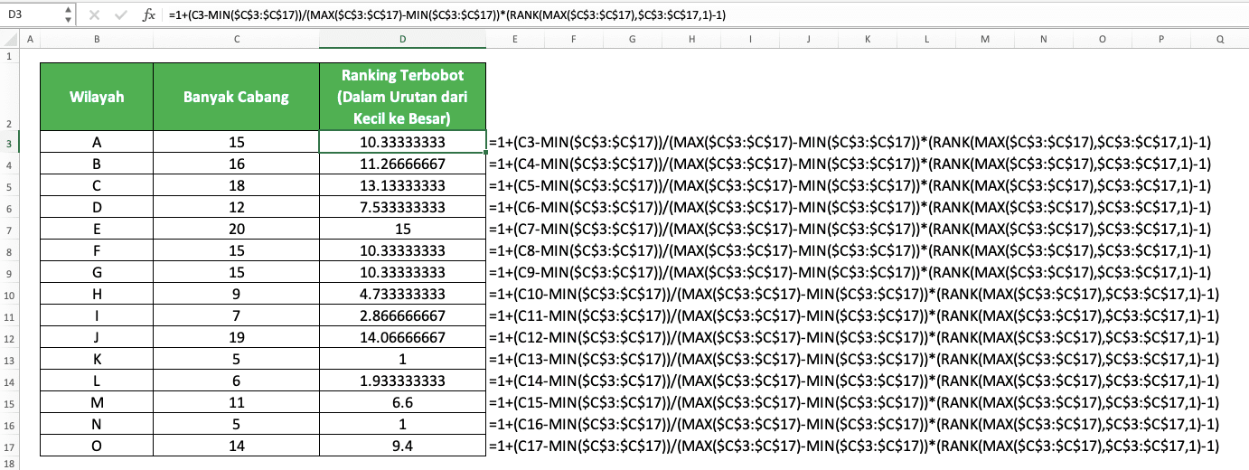
As we input the same number cell ranges to MAX, MIN, and RANK, we should input them using dollar symbols. This is so we can copy down our first formula writing without problem to get the weighted ranks for all numbers.
Write the formulas correctly using the concept we discussed and you should get your weighted ranks like in the example!
How to Do Dynamic Ranking in Excel
Does your numbers cell range keep adding new numbers and do you want your RANK formula to dynamically adjust to that? Well, for this, you should write an OFFSET and COUNTA combination as the numbers cell range input of your RANK.OFFSET is a formula that can move and/or stretch the cell/cell range we input into it. Meanwhile, COUNTA is a formula that can count the data amount we have in a cell range. By combining them as our RANK input, we can do a dynamic ranking that adjusts itself to new numbers we add!
The general writing form of the RANK, OFFSET, and COUNTA combination is as follows.
= RANK ( number_to_rank , OFFSET ( numbers_cell_range_first_cell , 0 , 0 , COUNTA ( extended_numbers_cell_range ) , 1 ) , [ order ] )
This formula writing assumes you want to rank numbers in a column cell range, not a row.
Here, we input the first cell of our numbers cell range as the cell we want to stretch using OFFSET. We use COUNTA as the row stretch input in the OFFSET. The cell range we input in COUNTA includes current cells with numbers and cells where we will input our new numbers.
By doing those, when we input new numbers into our column, OFFSET will stretch the numbers cell range input in RANK! Thus, the previous ranks for our numbers will automatically update themselves by considering the new numbers. If we need to rank the new numbers as well, we just need to copy our formula writing for them.
Here is the implementation example of the RANK, OFFSET, and COUNTA combination.

As you can see, we use a RANK, OFFSET, and COUNTA formulas combination to rank our numbers. We rank our numbers in descending order here. In the COUNTA, we input a cell range from our first number until the last row in our worksheet.
If we input new regions with their number of branches there, then our ranks will update themselves. This doesn’t happen if we just use RANK in our formula writing.
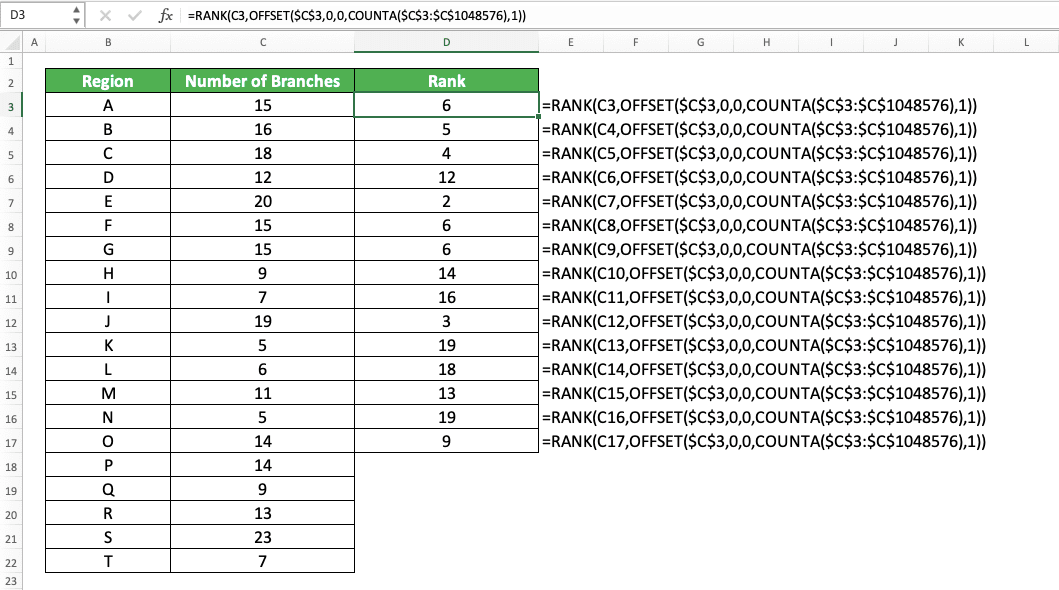
If we need the ranks of the new number entries too, we just have to copy down our formula writing.

Quite useful if you often need to update your numbers cell range, isn’t it?
How to Rank in a Pivot Table
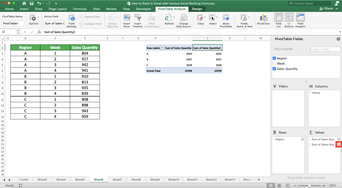
To rank the numbers in your pivot table, you should have the numbers labels and numbers ready in it. After that, you need to add your numbers as an additional value and turn it into the ranks you want.To better understand the concept, let’s see how we rank the numbers in the following pivot table.
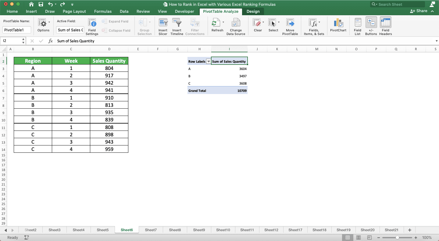
We created the pivot table from the data table we have on the left. We have the regions as our number labels and the sales quantities as our numbers. We put the regions as the Rows of our pivot table and the sales quantities as its Values.
To rank the sales quantities there, we add another sales quantities value in our pivot table fields.
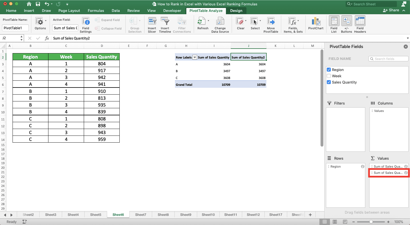
To turn the additional value into ranks, we click the value button to manage it.
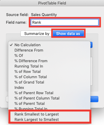
In the dialog box that shows up, give a clear name for your ranks like “Rank”. Then, go to the “Show data as” tab. Click the dropdown in the middle and choose “Rank Smallest to Largest” or “Rank Largest to Smallest” (depending on what order you want to base your ranks on).
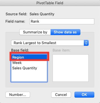
Next, in the Base Field box, choose your number labels. In the example, that means we should choose Region there.
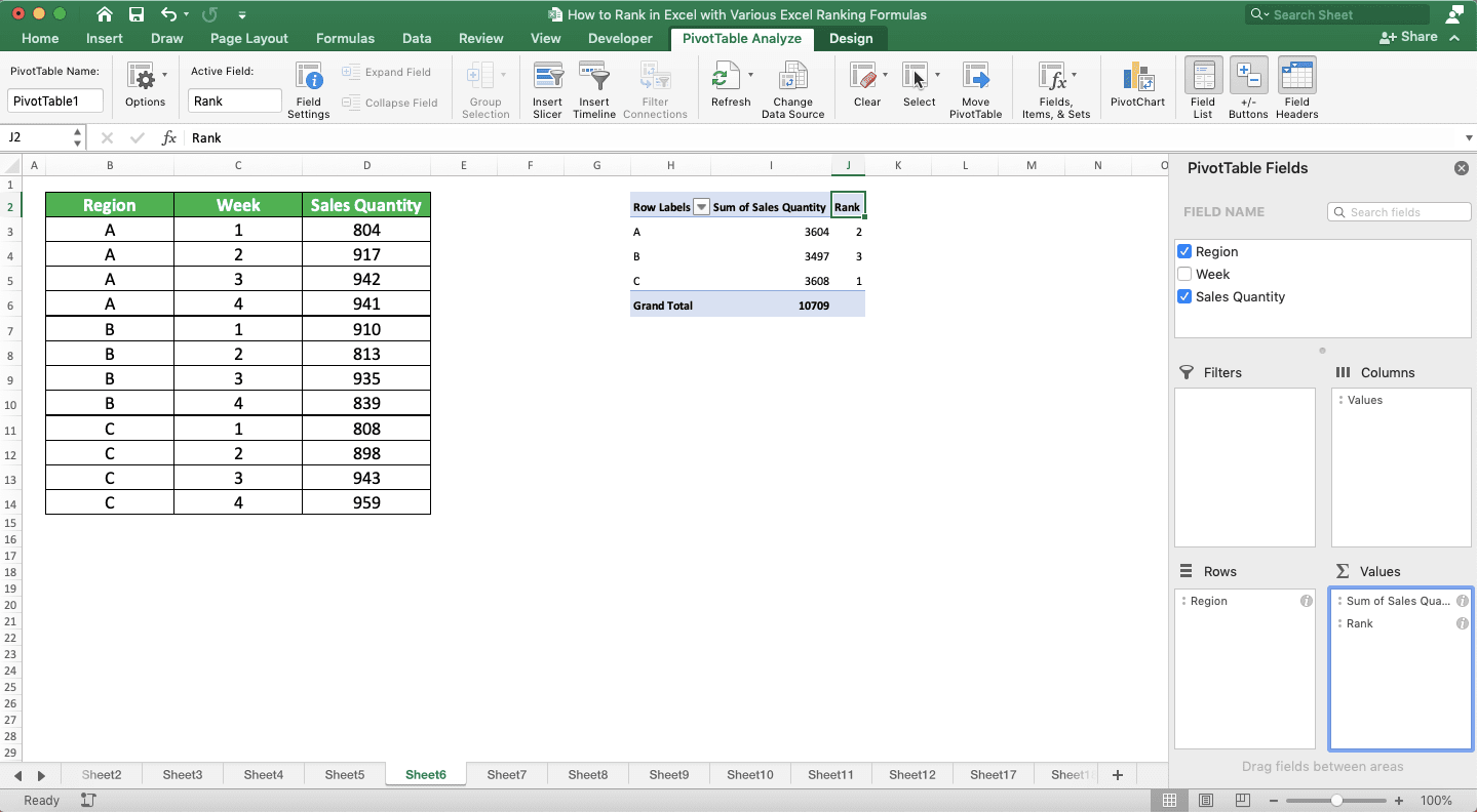
After you do all of that in the dialog box, click the OK button. You will immediately get the ranks of your numbers in your pivot table!
How to Get the Nth Largest/Smallest Value in Excel
Need to get the nth largest/smallest value from your numbers instead of their ranks? You can do that easily in excel since there are special formulas to do that kind of task. Those formulas are LARGE for the nth largest value and SMALL for the nth largest value.The general writing form of both formulas in excel is as follows.
LARGE
= LARGE ( numbers_cell_range , nth )
SMALL
= SMALL ( numbers_cell_range , nth )
Both formula writings are quite similar, aren’t they? Just input your numbers cell range and the order of the number you want to get to LARGE/SMALL.
Here is their implementation example in excel.

Here, we want to get the third largest and fifth smallest sales quantity from the monthly sales quantity data. To get those numbers, we use the LARGE and SMALL formulas.
Just input the sales quantity column cell range and the order of the number we want to LARGE/SMALL. In this case, we input three to LARGE and five to SMALL for the number order.
Write your LARGE/SMALL formula correctly and you will get the nth largest/smallest value you want!
Exercise
After you have learned how to rank in excel completely, now let’s do an exercise. Do it so you can practice what you have just learned and understand the lessons better.Download the exercise file below and answer all the questions. Download the answer key file if you have done the exercise and want to check your answers!
Link to the exercise file:
Download here
Questions
Answer each question in the appropriate gray-colored column according to their number!- Rank the inventory quantities normally in ascending order!
- Rank the inventory quantities according to their product in descending order!
- Rank the inventory quantities of warehouses II, VI, and VIII only in descending order!
Link to the answer key file:
Download here
Additional Note
You can also rank dates and times in excel as they are also a number data type. Just rank them using the methods you use to rank your numbers.Related tutorials you should learn:


