How to Insert a Tick Symbol/Checkmark in Excel

In this tutorial, you will learn how to insert a tick symbol/checkmark in excel.

Occasionally, we might need to create checkmarks for the work that we do in excel. We may sometimes want cross marks instead although we mostly use them to mark incorrectness.

There are several methods you can use to insert those marks in excel as you will see in this tutorial. From the method choices, you should choose the method you prefer that best fits your current data processing needs.

Want to know more about those methods and the way to master them? Learn from this tutorial until its last parts!

Disclaimer: This post may contain affiliate links from which we earn commission from qualifying purchases/actions at no additional cost for you. Learn more

Want to work faster and easier in Excel? Install and use Excel add-ins! Read this article to know the best Excel add-ins to use according to us!

How to Insert a Tick Symbol/Checkmark in Excel 1: Symbol Menu

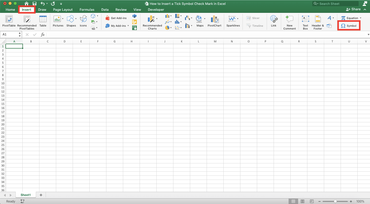
There are eight methods to insert a tick symbol/checkmark we will discuss in this tutorial. The first method is probably the most obvious one, the symbol menu.

Excel provides this symbol menu to input various kinds of symbols to your cell, including the checkmark one. To access this menu, just go to the Insert tab of your excel file and click the Symbol button there.



There will be a dialog box shows up. If you use excel in a Windows OS, then choose Wingdings from the font dropdown in that dialog box. Next, just find the checkmark symbol you want to insert into your cell (The symbol collection of the dialog box’s default font, Calibri, doesn’t have a checkmark. However, if you use Mac, then you can just find and click on the checkmark symbol you want to insert directly).



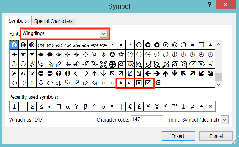
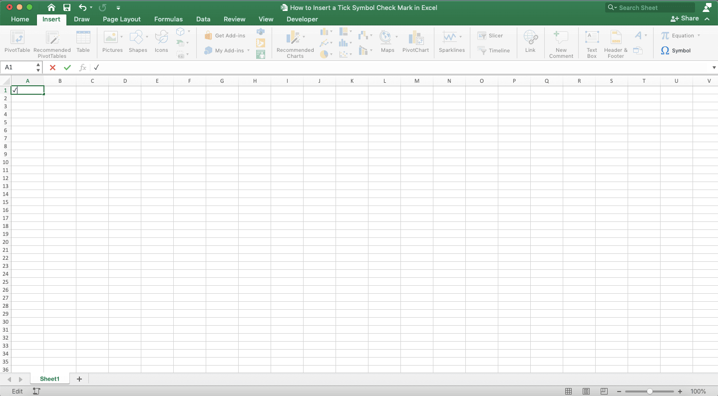
Choose the symbol by clicking on it and click Insert. You will automatically insert a checkmark or cross mark symbol to your current active cell!

How to Insert a Tick Symbol/Checkmark in Excel 2: Alt + Character Code

Another method to insert a tick symbol in excel is by pressing Alt + character code. The character code there is several numbers you press from the numeric keypad if you have it on your keyboard.

A numeric keypad is the number buttons on the right side of some types of keyboard, not the usual number buttons. If you have it, then just press the buttons below to get these results when your NUM LOCK is on.

Buttons	Result
Alt + 0252	A checkmark
Alt + 0254	A checkmark with a box
Alt + 0251	A cross mark
Alt + 0253	A cross mark with a box

Note that you can use those buttons to give you a tick symbol in Windows OS only. For Mac, you can press Option/Alt + V to get a form of checkmark instead (no need for a numeric keypad).

How to Insert a Tick Symbol/Checkmark in Excel 3: CHAR Formula

You can also use the CHAR formula to insert a checkmark or cross mark in your cell.

This CHAR method can be useful if you want the mark as a result of a formula that you write. Just write the CHAR formula as the result input part of your other formula if that is the case.



Just type the CHAR formula with the inputs like this to get the results you need.

CHAR Formula Writing	Result
=CHAR(252)	A checkmark
=CHAR(254)	A checkmark with a box
=CHAR(251)	A cross mark
=CHAR(253)	A cross mark with a box

252 and 254 are the code inputs for a checkmark while 251 and 253 are for a cross mark. Don’t forget to change your cell’s font family to Wingdings so you can get those symbols correctly.

You can use these codes for CHAR if you have your excel in a Windows OS. If your excel is in Mac, then you need to input 159 instead to get a checkmark from your CHAR. For a cross mark, input 158.

How to Insert a Tick Symbol/Checkmark in Excel 4: Shortcut Buttons

For this method to work well, you need to change the font family of your cell to Wingdings 2 or Webdings. These font families will turn the letters you write in your cell into symbols.

To create checkmarks or cross marks symbols in those fonts, here is what you should type.



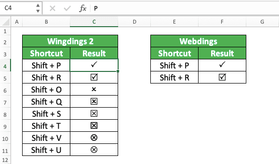
Pick the symbol form you like to input into your cell from those choices!

How to Insert a Tick Symbol/Checkmark in Excel 5: Copy-Paste

If you already have your checkmark/tick symbol somewhere in another cell, then you can just copy it. This method might be the easiest and fastest method to insert the symbol in your desired cell.

Just move your cell cursor to the cell containing the checkmark/tick symbol and press Ctrl + C (or right-click it and choose Copy). Then, move the cursor to the cell where you want to insert your symbol and press Ctrl + V (or right-click it and choose Paste). By doing that, you have inputted the tick symbol/checkmark you want to your designated cell!

How to Insert a Tick Symbol/Checkmark in Excel 6: AutoCorrect

You can also utilize the AutoCorrect feature in excel to insert your tick symbol. If you often need to insert the symbol in your current work, then this might be the best method to implement.

To run this method, you can follow these steps. First, insert the tick symbol you want in any cell using any method we discuss before. Then, copy the writing of the symbol to your clipboard.

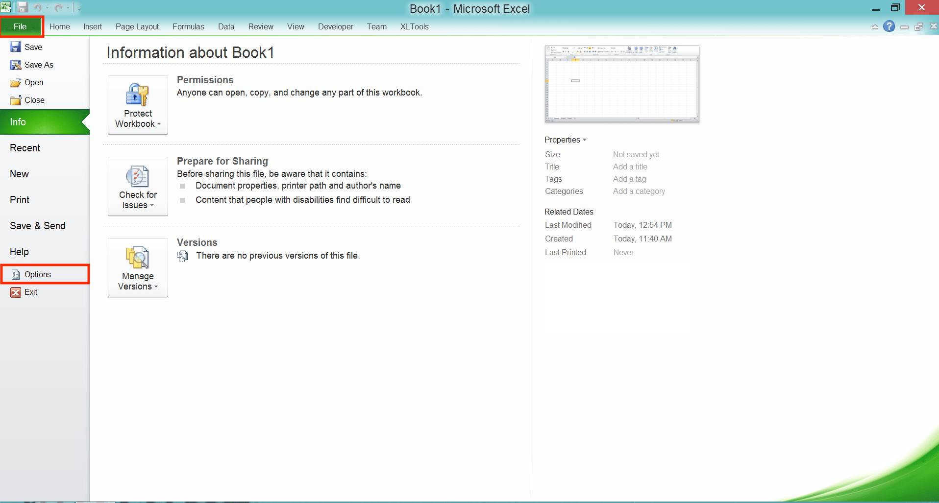
Next, click File and then Options (click Excel and then Preferences for Mac).



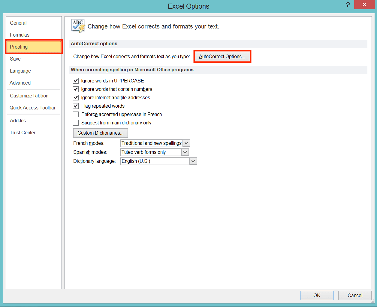
In the dialog box that shows up, click Proofing on the left side. After that, click the AutoCorrect Options button inside the Proofing menu on the right hand side (click AutoCorrect for Mac).



In another dialog box that shows up, do this. Type the text you want as a trigger to insert your tick symbol in the Replace text box. In the With: text box, paste the tick symbol you have copied in your clipboard. Click Add after that.



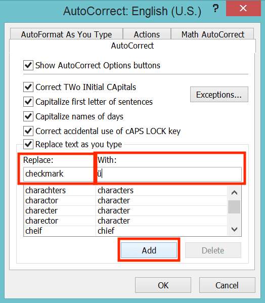
Click OK. Now, every time you type the trigger word, excel will immediately transform it to your tick symbol! Don’t forget to change the font type to Wingdings where you input your trigger word to get the tick symbol correctly!

How to Insert a Tick Symbol/Check Mark in Excel 7: Insert Image

Another method you can use to insert a tick symbol/checkmark in excel is by inserting the symbol image.

Have the image file of the tick symbol/checkmark ready at your computer (you can find many choices in the internet). Then, just go to the Insert tab and click the Picture button.



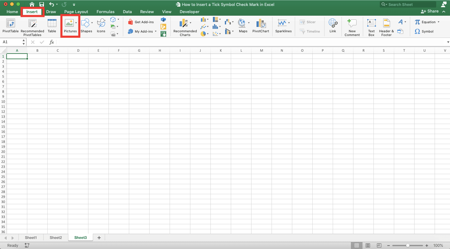
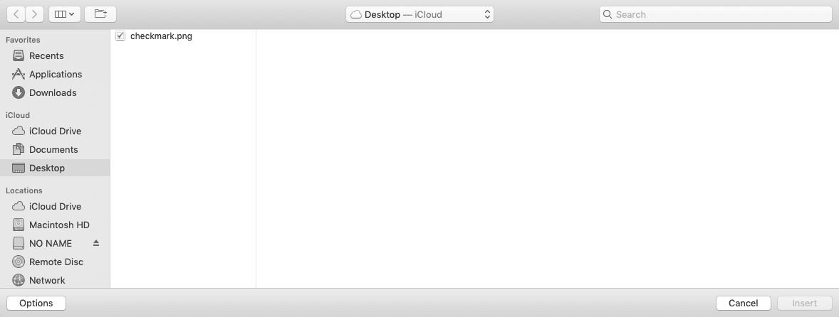
Locate where your tick symbol/checkmark image file is. Then, double click it or choose it and click Insert.



Doing that will insert the tick symbol/checkmark image into your worksheet.



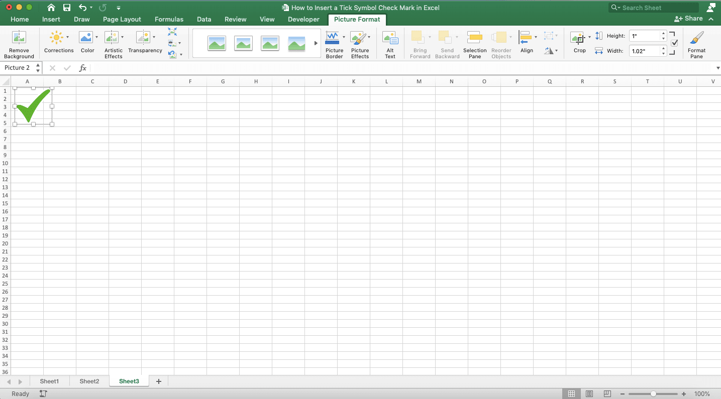
Adjust the image to your preference so it can display itself the way you want.

How to Insert a Tick Symbol/Checkmark in Excel 8: Conditional Formatting

The last method we are going to introduce is by using conditional formatting. If you have some criteria to mark the data in your cells with checkmarks, then this is the method for you.

To understand how to use this method easier, take a look at the following example. Let’s say we have this data in our worksheet that we want to give check marks on.



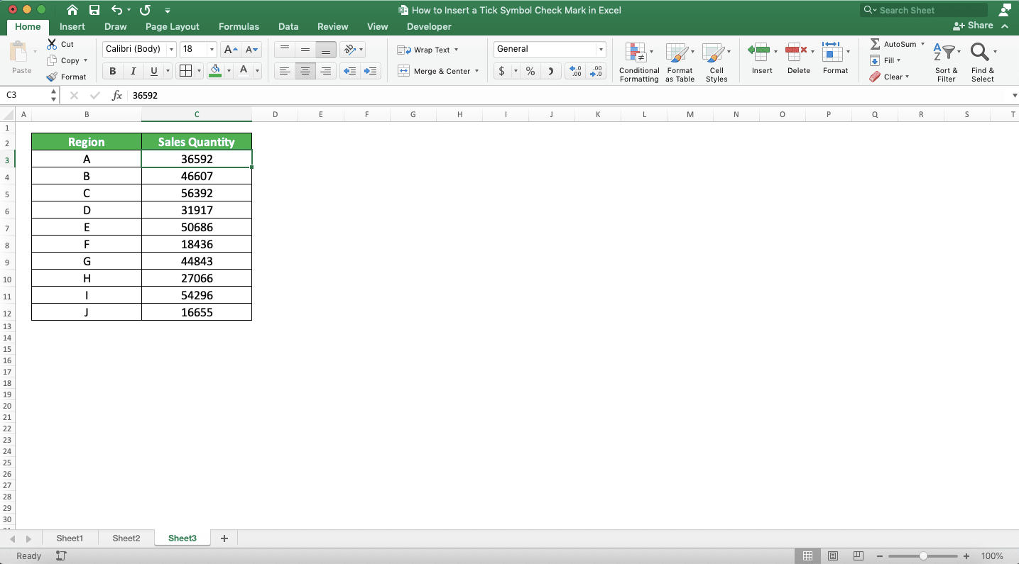
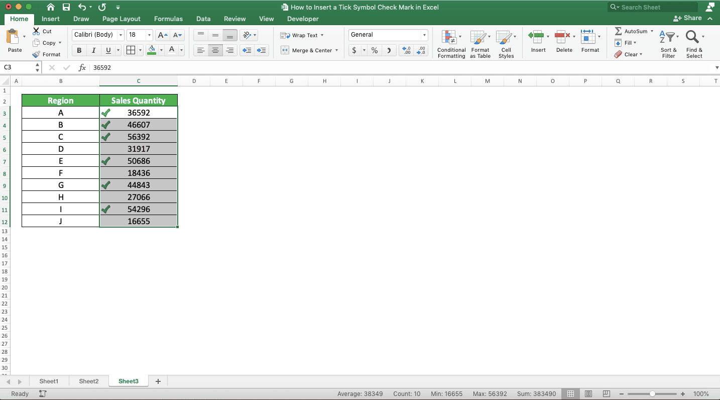
We want to mark all the sales quantities above 35000 with checkmarks. We can do that easily if we use the conditional formatting method.

First, highlight the cell range where you want to put your checkmarks. Next, click the Conditional Formatting dropdown in the Home tab and choose New Rule….



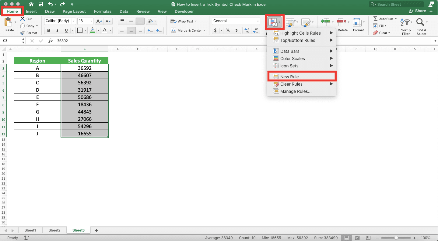
In the dialog box that shows up, choose Format all cells based on their values rule type. Then, in the Format Style dropdown, choose Icon Sets.



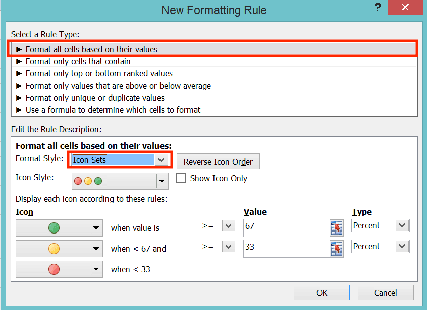
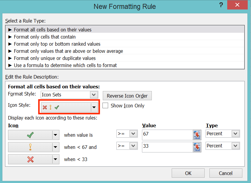
In the Icon Style dropdown, choose the icon style which has a checkmark form you want in it. After that, you can set the rule where you want the checkmark to show up.



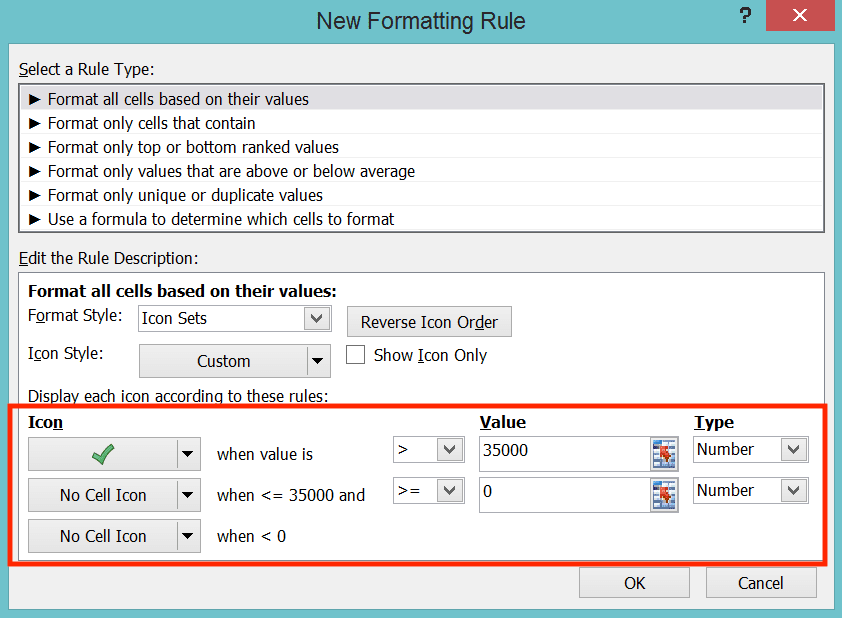
For this example, we set the rule so the checkmark will show up if the cell value is above 35000. We give no icon if the cell has another value.



After you have set the rules, click OK. The checkmarks will show up on the cells with values that correspond to your rule!

Format a Tick Symbol/Checkmark in an Excel Cell

If the tick symbol you insert is in your cell (you use method 1-6 to insert it), then you can format it just like any other text. You can change its color, font size, bold/italic/underline it, and do other things like that.

This is as you can see the example below. We give our checkmark a blue color, 32 font size, and bold style here.



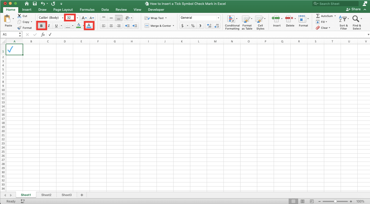
If your tick symbol is an image, then you can format it just like any other image too in excel. If your tick symbol is from conditional formatting, however, then you cannot change its format (you must follow the format given by the conditional formatting).

Conditionally Format Cells Based on Tick Symbols/Checkmarks

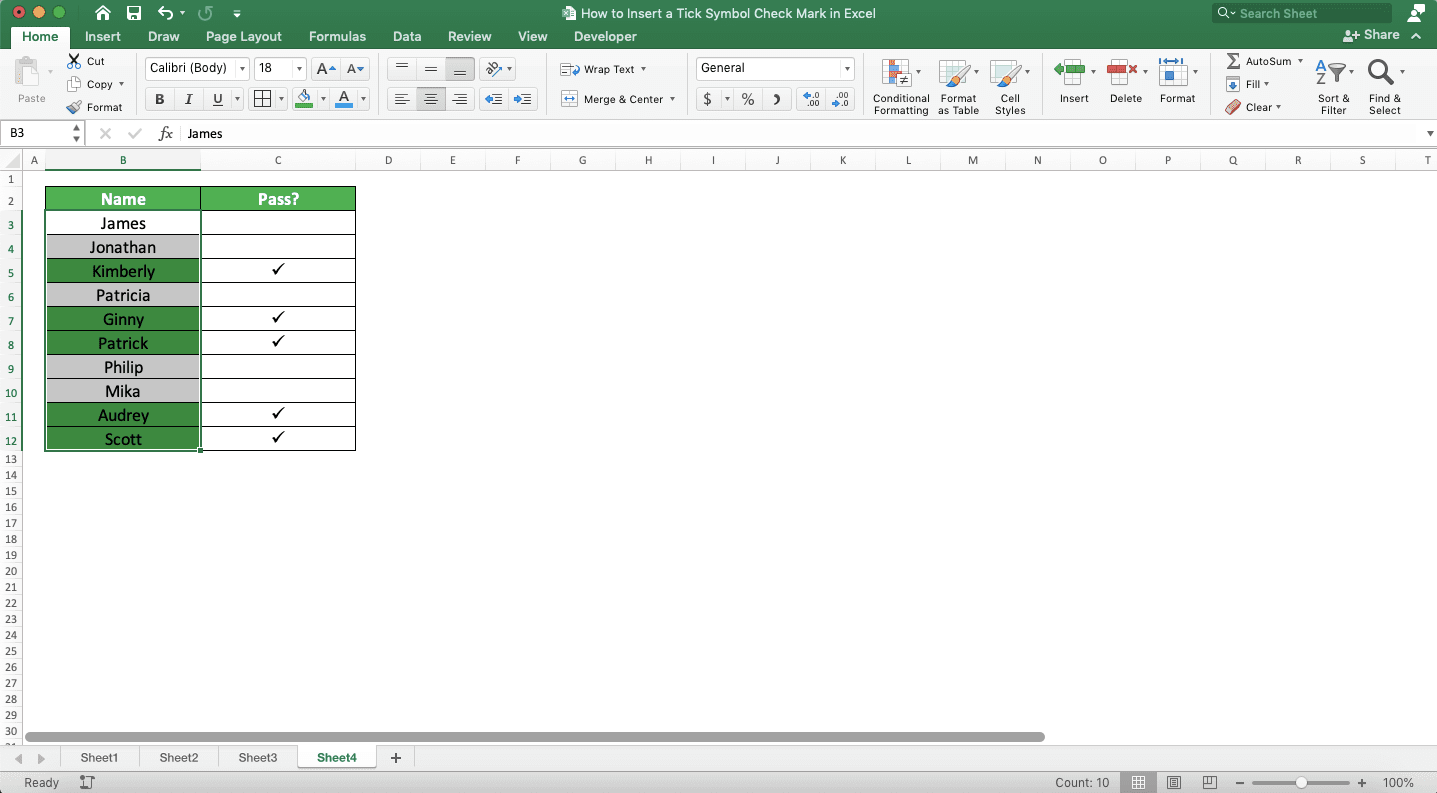
If your tick symbols are from CHAR formulas or Wingdings 2/Webdings font, then you can conditionally format based on them. Just use the formula rule which compares your cell values to what you use to create the tick symbols. Your cells need to only contain the tick symbols for this to run optimally.

To understand the concept easier, let’s see an example. We have this data and we want to mark the name who passes with green cell colors.



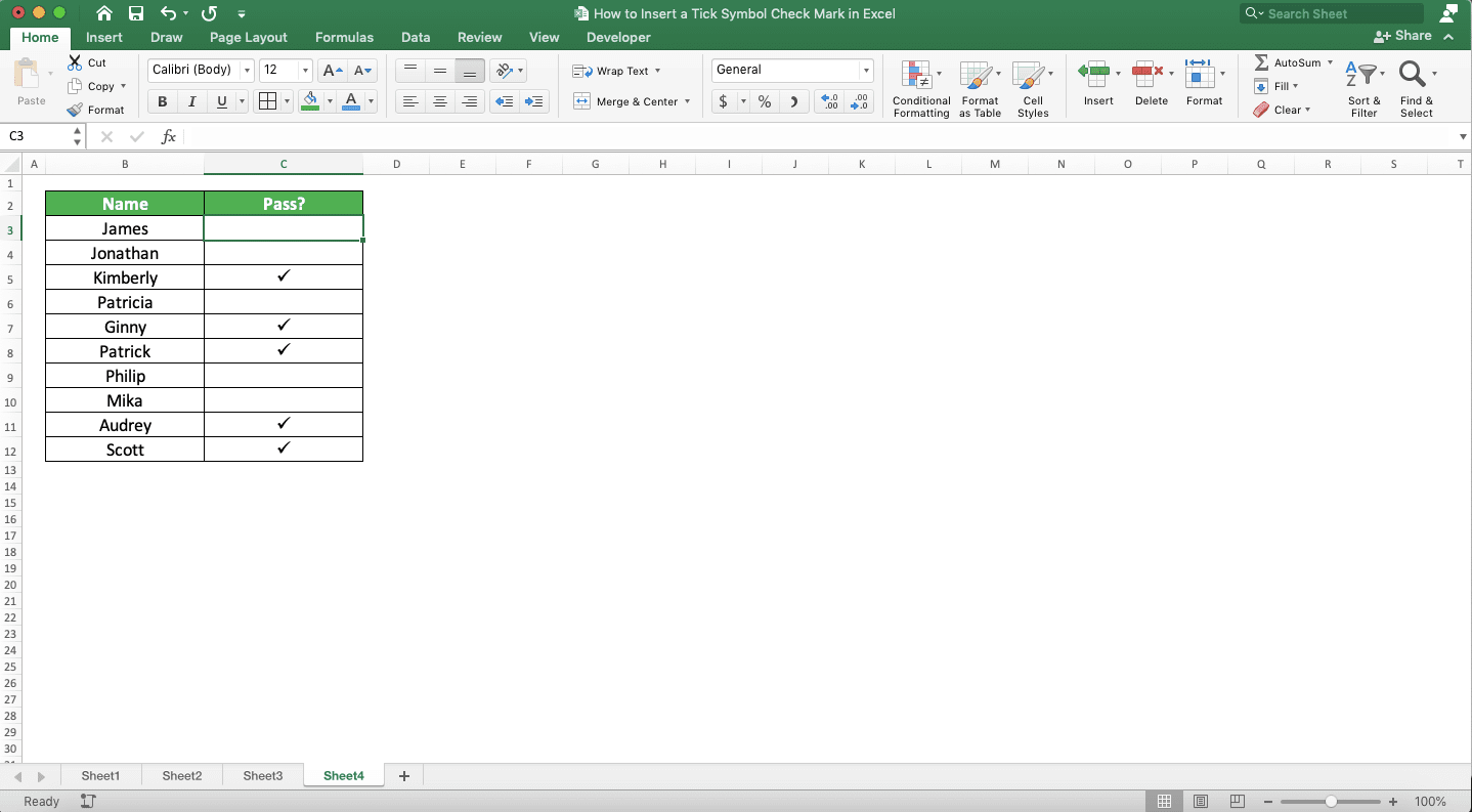
What to do? Well, as we create the checkmarks to indicate the pass results there with the CHAR formula, we can use conditional formatting.

Highlight the cells where you want to conditionally format and choose New Rule… in the Conditional Formatting dropdown in Home.



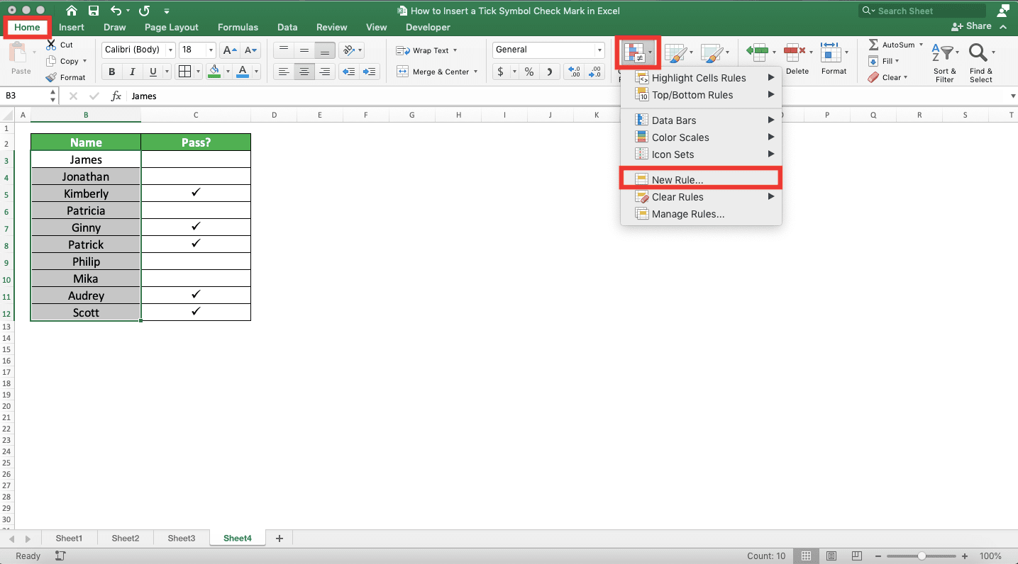
In the dialog box that shows up, choose the Use a formula to determine which cells to format rule type. Then, write a formula that equals the corresponding cell which might contain a checkmark with the way you write your checkmarks.

As we use CHAR to create our checkmarks in the example, we write =$C3=CHAR(252) in the text box (if you use Wingding 2/Webdings, then write the shortcut letter you use to create your checkmarks as the comparison value). Don’t forget to remove dollar symbols in front of the row/column coordinate when appropriate.



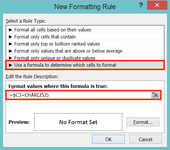
Don’t forget to set the cell format if the corresponding cell contains a checkmark by clicking the Format button there. For this example, we want the name cell to be green if the checkmark is there.



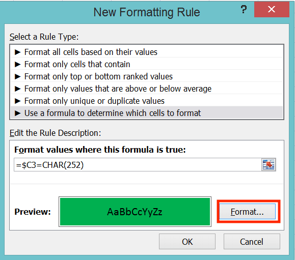
Click OK and you have conditionally formatted your cells based on the checkmarks!

Count Tick Symbols/Checkmarks in a Cell Range in Excel

To count the tick symbols in a cell range, you must also have created them using CHAR or Wingdings 2/Webdings. It is because we need the CHAR and Wingdings 2/Webdings shortcut as the criteria of our counting process.

We use COUNTIF as the formula to get the number of our tick symbols. If you use the symbols as one of your several counting criteria, then you should use COUNTIFS instead.

Here is the COUNTIF writing to count tick symbols in a cell range (for COUNTIFS, you just need to give the inputs as one of your COUNTIFS input pairs).



Input the CHAR or shortcut criterion in the COUNTIF, depending on using what you created your tick symbols previously.

Here is the example of the COUNTIF implementation in excel to do the counting process. We use the same data as the one we use in the previous tutorial part.



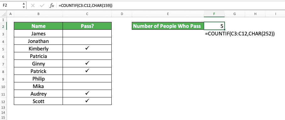
We input the CHAR(252) criterion because we use the CHAR formula to create our checkmarks there. As you can see, it enables COUNTIF to count the right number of checkmarks, which is 5.

Additional Note

If you use Windows, then you can see a symbol code for your CHAR input in the Symbol menu dialog box. You can see the location where you can see in the screenshot below (in the red box).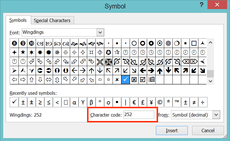



Just select the symbol in the dialog box and you can see the code there. This is handy when you forget what you should input when you use the CHAR formula to get a tick symbol.



Related tutorials you should learn: