HLOOKUP Formula in Excel: Functions, Examples, and How to Use
Home >> Excel Tutorials from Compute Expert >> Excel Formulas List >> HLOOKUP Formula in Excel: Functions, Examples, and How to Use


In this tutorial, you will learn how to use the HLOOKUP formula in excel completely.
When we work in excel, we sometimes need to find information from a reference table. We usually use VLOOKUP for this but VLOOKUP can only do its lookup process vertically (find data by looking in a cell range by column). When we need to look for data horizontally, HLOOKUP can be the solution to help us with the process.
Want to master the usage of the HLOOKUP formula? Learn from this tutorial until its last part!
Disclaimer: This post may contain affiliate links from which we earn commission from qualifying purchases/actions at no additional cost for you. Learn more
Want to work faster and easier in Excel? Install and use Excel add-ins! Read this article to know the best Excel add-ins to use according to us!
Table of Contents:
- What is HLOOKUP?
- HLOOKUP function in excel
- HLOOKUP result
- Excel version from which we can start using HLOOKUP formula in excel
- The way to write it and its inputs
- Approximate vs exact match in HLOOKUP
- HLOOKUP example: usage and result
- Writing steps
- Common factors why HLOOKUP produces an error/wrong result + solutions
- Difference between VLOOKUP and HLOOKUP in excel + example
- HLOOKUP with multiple criteria
- HLOOKUP from another sheet
- HLOOKUP from another workbook
- Lookup data in a dynamic row: HLOOKUP MATCH
- Case-sensitive HLOOKUP
- HLOOKUP with wildcard characters
- A better alternative to HLOOKUP? HLOOKUP vs INDEX MATCH
- Exercise
- Additional note
What is HLOOKUP?
We can define HLOOKUP, an abbreviation of horizontal lookup, as a formula to find data horizontally in a cell range. Horizontally here means HLOOKUP will find the data by looking for it at the cell range by row.HLOOKUP Function in Excel
We can use HLOOKUP to get data from a cell range that categorizes its data using rows.HLOOKUP Result
From HLOOKUP, we can get the data we look for from a cell range.Excel Version from Which We can Start Using HLOOKUP Formula in Excel
We can start using HLOOKUP since excel 2003.The Way to Write It and Its Inputs
Generally, we can write HLOOKUP in excel like this.
= HLOOKUP ( lookup_reference , reference_cell_range , result_row_index , lookup_mode )
Here is a bit explanation of each input in the writing.
- lookup_reference = the reference value that HLOOKUP will try to find in our cell range’s first row to get our data column position
- reference_cell_tange = the cell range where we will look up for the data that we want
- result_row_index = the index of the row in the cell range we input where HLOOKUP should get our data from
- lookup_mode = optional. Determines whether HLOOKUP will try to find an exact or appropriate match of our lookup reference value. Input TRUE for approximate or FALSE for exact. If we don’t input anything here, then HLOOKUP will assume the input is TRUE
Approximate vs Exact Match in HLOOKUP
Let’s talk more about the nature of approximate or exact match in HLOOKUP as people often get confused with it.We can set the approximate or exact match lookup mode in HLOOKUP at the last part of its input. We input TRUE if we want an approximate match and FALSE if we want an exact match. This is an optional input and the default is TRUE.
However, what does it mean by approximate or exact match? If you use the approximate match, then this is what happens. If HLOOKUP doesn’t find an exact match for your lookup reference value, then it will get its smaller nearest value.
If you use the exact match, however, then HLOOKUP will produce an error if it doesn’t find the exact match.
Does that mean it is always better to use an approximate match since it has a smaller error possibility? Well, you must pay attention to two things before you decide to use the approximate match lookup mode.
First, you may only want to get an exact match for your reference value when using your HLOOKUP. This is because a smaller nearest value to it may make you find the wrong data. In this situation, you may want to combine your HLOOKUP with IFERROR to substitute the error if that happens.
Second, if you use an approximate match, then you should sort the first row of your cell range in ascending order. If you don’t, then HLOOKUP can produce a wrong result or even an error!
So, which HLOOKUP lookup mode you should choose? After you learn the explanation from this tutorial part, choose the best one depending on your data processing situation!
As an additional note, this approximate and exact match explanation also applies to VLOOKUP if you use the formula.
HLOOKUP Example: Usage and Result
The following will give and explain the example of HLOOKUP implementation in excel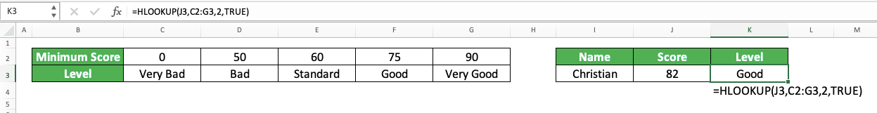
From here, we can see the writing and result example of HLOOKUP. As explained before, this formula needs the inputs of lookup reference, cell range, and the row index to get the result. The TRUE/FALSE part at the end of its writing is optional.
To find your data, HLOOKUP will search its reference value in the first row of your cell range. It will have its result from the row with the index that you input.
When HLOOKUP finds the reference value in the first row, it will retrieve its column position. If there is more than one match, then HLOOKUP will retrieve the column position of the most left match.
If you understand the example, then you should be able to understand how the formula works too. We use TRUE there so HLOOKUP can do its lookup process based on the approximation of its reference value.
The reference value here is 82. Because there is no 82 in the first row, it will take the smaller nearest value to 82, which is 75.
The 75 column then lines up with the row which index we input earlier (our input here is 2 which means the second row of the cell range). From the second row and the 75 column, we get the “Good” result. This “Good” then becomes the HLOOKUP result in the example!
Writing Steps
The following part will discuss how to write the HLOOKUP formula in excel step-by-step.We will discuss each step with an example in the form of a screenshot. This is so you can understand the explanation easier.
-
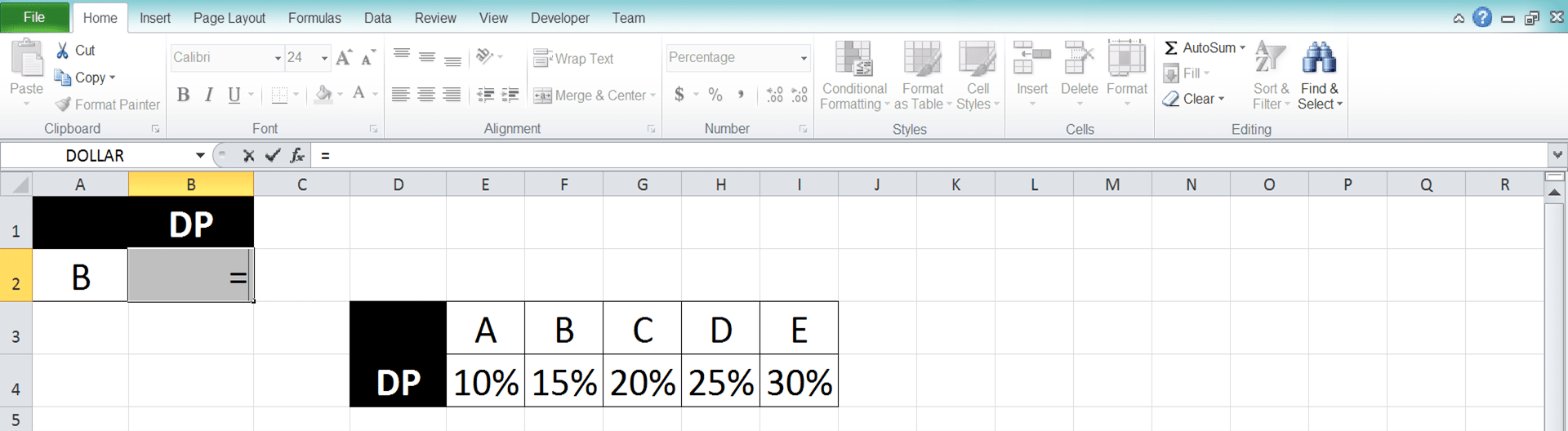
Type an equal sign ( = ) in the cell where you want to put your HLOOKUP result
-
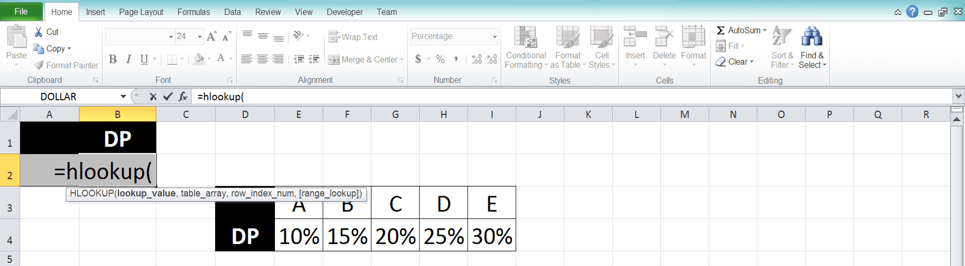
Type HLOOKUP (can be with large and small letters) and an open bracket sign after =
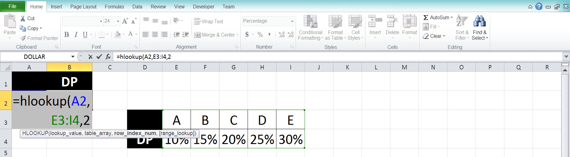
-
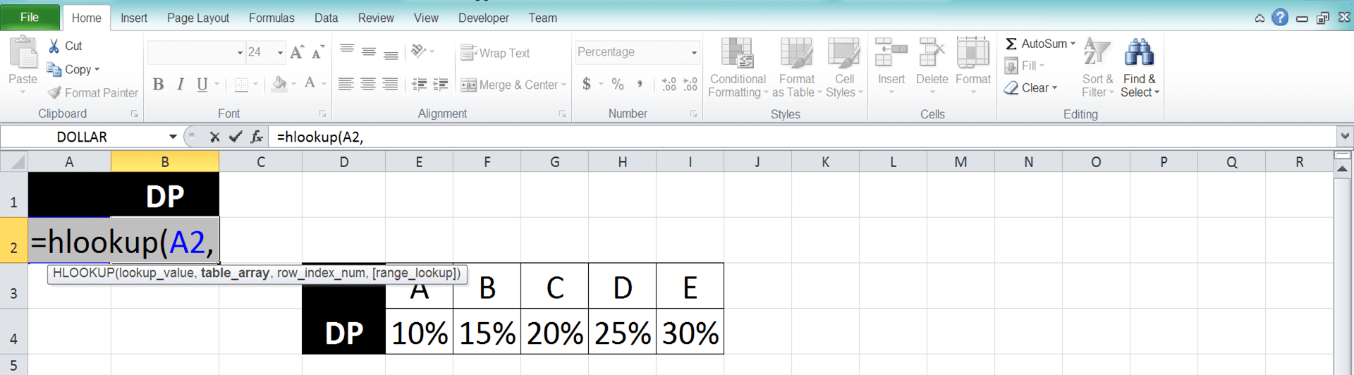
Input the lookup reference value or cell coordinate where the value is. HLOOKUP will try to find this value in its cell range’s first row as a way to get its result. Then, type a comma sign ( , )
-
Input the cell range where your reference table is (where you want to get your data). Then, type a comma sign

-
Input the nth order of the row (row index) where HLOOKUP should get its result in your reference table. HLOOKUP will get the result from the column in which it finds your lookup reference value and in this row too. If there is more than one match for the lookup reference value, it will take the match on the most left
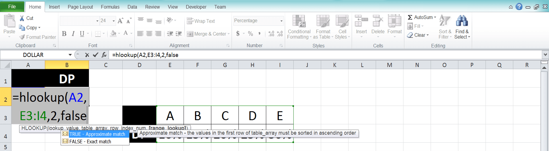
-
Optional: To determine whether HLOOKUP should find an exact or approximate match for your lookup reference value, do this. Type a comma sign and input TRUE/FALSE (can be with large and small letters). TRUE for an approximate match and FALSE for an exact match.
The approximate match definition is if there is no exact value, then HLOOKUP will do this. HLOOKUP will take the smaller nearest value from the lookup value in the reference table’s first row as a reference. However, you must sort the value in the first row in ascending order so the TRUE input functions correctly.
If there is no input from you in this part, then HLOOKUP will assume the input as TRUE
-
Type a close bracket sign
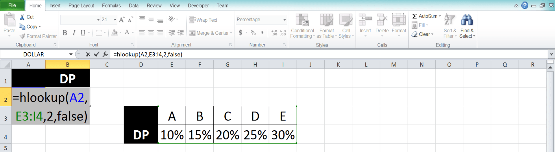
- Press Enter
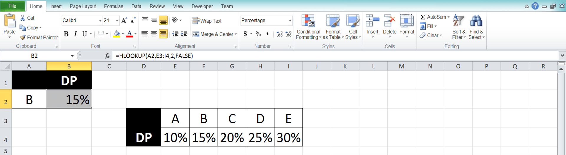
-
Done!
Common Factors Why HLOOKUP Produces an Error/Wrong Result + Solutions
Got a wrong result or even an error from your HLOOKUP? There can be many factors that cause this to happen. However, these factors below are probably the most possible ones. We also discuss the solutions you can use to fix those factors below.- Factor: You input TRUE (or don’t input anything) for the search mode of your HLOOKUP. However, you haven’t sorted the first row of your reference table in ascending order. Solution: Sort the first row of your reference table in ascending order. If you are fine in just finding an exact match of your lookup reference value, then input FALSE instead.
- Factor: Your lookup reference value is in a row other than the first row of your reference table. Solution: Adjust your cell range input so HLOOKUP can find your lookup reference value in the first row of it. Alternatively, you can also move the row that contains the lookup reference to the first row of your cell range.
- Factor: You input the wrong row index to retrieve your HLOOKUP result. Solution: This problem sometimes happens when you have a large reference table. Check again your result row index input to make sure you don’t input the wrong index. If it is wrong, then replace it with the right one.
Check again your HLOOKUP for these three points if you don’t get the result you want!
Difference Between VLOOKUP and HLOOKUP In Excel + Example
Although VLOOKUP and HLOOKUP are both data lookup formulas in excel, they have some big differences you should understand. You can read the summary of those differences in the table below.| VLOOKUP | HLOOKUP |
|---|---|
| Stands for “Vertical Lookup” | Stands for “Horizontal Lookup” |
| Look for data in a reference table based on columns | Look for data in a reference table based on rows |
| Find its lookup reference value in the first column of your reference table | Find its lookup reference value in the first row of your reference table |
The following gives the implementation example of VLOOKUP and HLOOKUP. You can see the differences between both from the reference table form and their inputs.
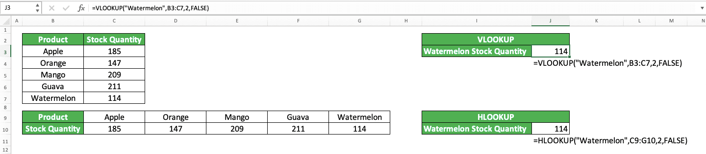
As you can see in the example, we should use VLOOKUP and HLOOKUP for different forms of reference tables. That is because VLOOKUP will look for data based on columns while HLOOKUP will do it based on rows.
For VLOOKUP, the reference table divides its data categories into columns while HLOOKUP’s reference table divides them into rows. Pay attention to the form of your reference table before deciding whether to use VLOOKUP or HLOOKUP.
Implement VLOOKUP or HLOOKUP correctly to get the correct data you need from your reference table!
HLOOKUP with Multiple Criteria
When using HLOOKUP, we usually only have one criterion (lookup reference value) to base our data lookup process on. But what if we have multiple criteria? Can we still use HLOOKUP to help us?The answer is yes, you can still use HLOOKUP. However, you need to add a “helper” row in your reference table to help you.
In the “helper” row, you concatenate relevant data from your reference table to accommodate your multiple criteria HLOOKUP. You can concatenate them using CONCATENATE/CONCAT (you can use CONCAT since excel 2019) formulas or by using the ampersand symbol ( & ).
Here are the general writing form of each concatenation method.
CONCATENATE
= CONCATENATE ( data1 , data2 , … )
CONCAT
= CONCAT ( data1, data 2 , … )
Ampersand symbol
= data1 & data2 & …
Make sure the “helper” row becomes the first row in your HLOOKUP cell range so your HLOOKUP can process it.
You should also concatenate the lookup criteria input in your HLOOKUP so it matches the data in your “helper” column. Here is the general writing form of HLOOKUP with multiple criteria to make you understand the concept better.
= HLOOKUP ( criterion1 & criterion2 & … , reference_cell_range , result_row_index , search_mode )
We concatenate our criteria in the lookup reference input part of our HLOOKUP to accommodate them in our data lookup process. Meanwhile, we give other inputs to our HLOOKUP normally. If you input TRUE for the search mode, then you should sort your “helper” row in ascending order.
To better understand this HLOOKUP with multiple criteria concept implementation, let’s take a look at the example below.
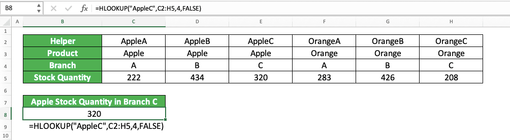
In this example, we have two lookup references to get our stock quantity from, product name and branch. To lookup data with multiple criteria like this, we can use HLOOKUP with the writing form we discussed earlier.
We add a helper row there and make it the table reference’s first row to help us in our HLOOKUP process. In the HLOOKUP, we concatenate our lookup references using direct typing and input the reference table which includes the helper row.
We use FALSE in the HLOOKUP because we need to find an exact match to our concatenated lookup reference. We do those things and we will get our HLOOKUP result by using multiple criteria/lookup references!
HLOOKUP from Another Sheet
If you have your HLOOKUP reference table in another sheet, then add that sheet name when you refer to it. However, if you have already named the table using the name manager feature, then you can refer to that name directly.To add the sheet name when referring to your HLOOKUP reference table in another sheet, here is the general writing form. You can write it manually or go to the reference table sheet and drag across the table to input it automatically.
‘ sheet_name ‘ ! reference_table_range
To refer to a reference table that already has a name, you just need to type the table name.
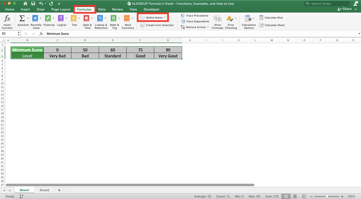
Need to know how to name your reference table using the name manager? First, highlight the reference table cell range. Then, go to the Formulas tab and click the Define Name button.
Just enter the name you want to give in the text box given in the dialog box that shows up. Then, click OK.
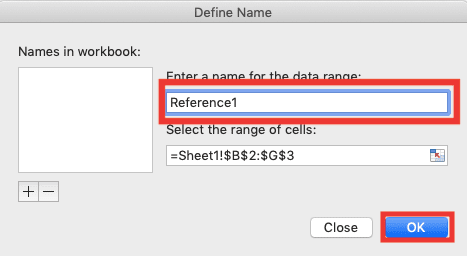
Now, you can use the name you gave to refer to the reference table!
To understand the concept of writing HLOOKUP by using a reference table in another sheet, here is the implementation example.
For this example, we have our reference table in a sheet with the name “Sheet1”
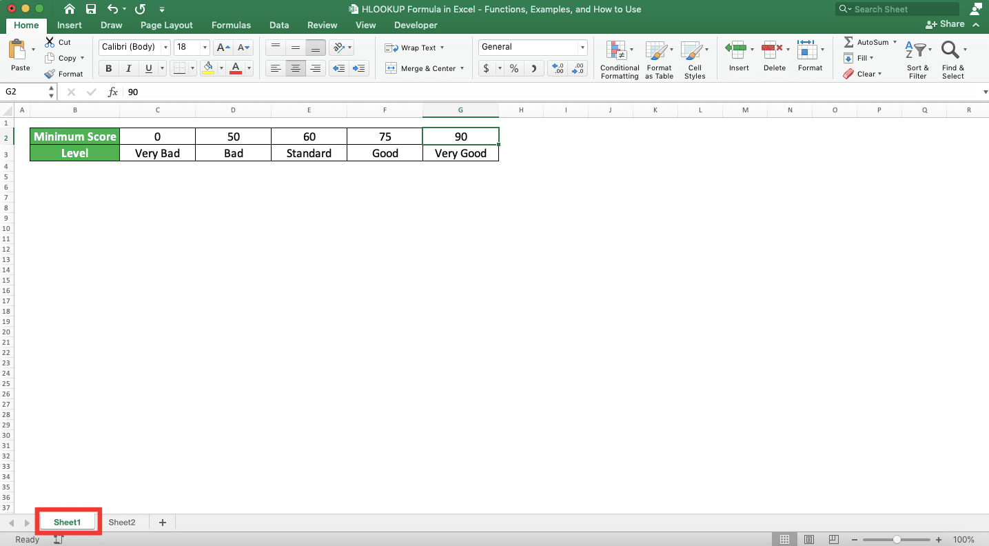
And we want to write our HLOOKUP in another sheet, “Sheet2”

What to do in this situation? Just write the HLOOKUP with the cell range input we discussed earlier!
For this example, we add the sheet name when inputting our reference table cell range to HLOOKUP.

Simple, isn’t it? In this example, we don’t use quote signs when writing the sheet name because the name doesn’t have spaces in it (if you write it using quote signs, then excel will automatically remove the quote signs if the name doesn’t have spaces).
Refer to the reference table in another sheet correctly and you will get your HLOOKUP result!
HLOOKUP from Another Workbook
If your HLOOKUP reference table is in another workbook, then write the workbook name when referring to the reference table. If you currently don’t open the workbook, then you need to write the file path to the workbook as well.You can also use the name manager to name the reference table for an easier reference process. Don’t forget the workbook name and its file path too when creating the name for the reference table cell range.
Here is the general writing form for the cell range of a reference table in another workbook in HLOOKUP.
‘ file_path [ workbook_name ] sheet_name ‘ ! reference_table_range
To make it easy to write it, open the reference table workbook when you write your HLOOKUP.
Drag your cell cursor across the reference table when you need to input it in your HLOOKUP. Excel will automatically add its file path when you close the reference table workbook.
To better understand the concept of HLOOKUP from another workbook, take a look at this example.
Let’s say we have our reference table in a workbook with the name “Reference Table” like this.
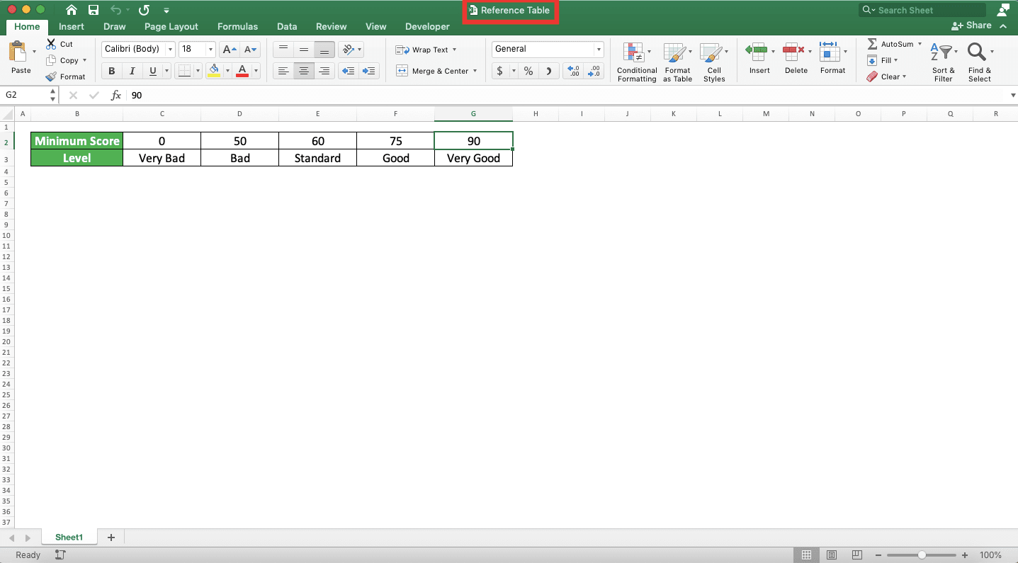
We want to refer to it in an HLOOKUP that we write in another workbook.

What to do so we can do that? Just input the reference table cell range using the form we have discussed earlier! For the example, that means we write our HLOOKUP with the input like this.

We write this HLOOKUP when we open the “Reference Table” workbook. If we close it, then excel will add its file path automatically!
Lookup Data in a Dynamic Row: HLOOKUP MATCH
Still don’t know which row index you want to get your HLOOKUP result from? Want to make it dynamic depending on the HLOOKUP header name you want at the time? You can combine your HLOOKUP with MATCH for that purpose.Here is the general writing form of the HLOOKUP and MATCH formulas combination in excel.
= HLOOKUP ( lookup_reference , reference_cell_range , MATCH ( result_row_header , row_header_cell_range , 0 ) , lookup_mode )
As we want the result row index input to be dynamic, we write MATCH in that HLOOKUP input part. We input the cell range where the row headers of our reference table are to our MATCH.
For the MATCH result_row_header input, we should input a cell reference. This is so we can just change the cell value whenever we need to change the result row index. We also input 0 to the MATCH because we want an exact match when finding the header position we want.
To better understand the HLOOKUP with the dynamic row concept, here is its implementation example.
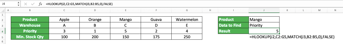
Here, we implement HLOOKUP with a dynamic result row by combining its writing with MATCH. You can see that it will change its result when we change the data we want to find.
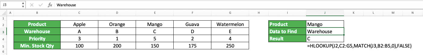
You can see how we write the HLOOKUP and MATCH combination in the screenshot. Input the cell value containing the row header name you want to see the data of to your MATCH. Also, input the row header cell range in your reference table there plus the 0.
Write your formula correctly and you can get a dynamic result from your HLOOKUP!
Case-Sensitive HLOOKUP
By default, HLOOKUP isn’t case-sensitive when it tries to find your lookup reference value. This means that it won’t differentiate between, for example, “Apple” or “APPLE” or “apple”. When you need to do a case-sensitive search, however, this HLOOKUP default nature can be troublesome. Take a look at the example below to better understand the impact of this matter.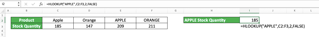
In the example, we have a stock quantity database in which we differentiate the product quality by letter capitalization. We capitalize all the letters of the product with the highest quality and count its stock differently too.
When we need to retrieve the stock quantity of the APPLE product name using HLOOKUP, we run into trouble. That is because HLOOKUP cannot differentiate between capital and small letters. As a result, it gives the stock quantity of Apple instead of APPLE (HLOOKUP will take the most left match in case there is more than one match for the lookup reference value).
So, what we can do if we need to be case-sensitive with our HLOOKUP just like the example above?
It is a bit complex but we can combine our HLOOKUP with MATCH, EXACT, and array formula to solve the problem. We need to also create a helper row containing our data number index and make it the first row.
Here is the general writing form of the formulas’ combination.
{ = HLOOKUP ( MATCH ( TRUE , EXACT ( lookup_reference_range , lookup_reference ) , 0 ) , reference_cell_range , result_row_index , FALSE ) }
To understand better about the writing, here is its implementation on the example we had earlier.
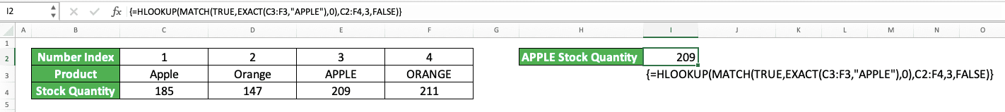
Using the method we discussed earlier, we can get the APPLE stock quantity through HLOOKUP. As we use the array formula form here (the curly bracket signs that envelop our formula writing symbolizes this), we need to press Ctrl + Shift + Enter when we finish writing our formula. Don’t just press Enter as usual because it will cause our formula writing to produce an error.
And here is the explanation of the process that happens through the formula writing if you want to understand it (you should if you have the time). First, we create a number index row to become the first row of our reference table before we write our formula. We need the row because our HLOOKUP lookup reference value will be the number index of our original lookup reference value.
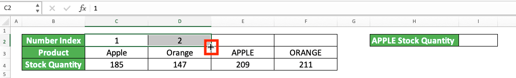
If you have a table reference with many columns, use the autofill feature to quickly fill the number index row. To use it, type 1 and 2 for the first two columns of the row and highlight their cells. Then, move your pointer to the bottom right of your cell cursor until it becomes a plus sign ( + ).
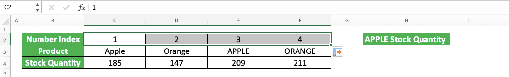
Click and drag to the most right column in your number index row. Release the drag and excel will automatically fill the number index row for you.
After we finish creating the number index row, we start writing our formula. We write MATCH as our HLOOKUP first input because we need the number index of our lookup reference there.
In MATCH, we write TRUE as the lookup reference as we will get a TRUE and FALSE array from our EXACT. We get a TRUE and FALSE array because we input a cell range into EXACT (this is also why we use an array formula form, because EXACT usually accepts individual inputs not a cell range) with our original lookup reference value. The cell range is the row cell range from our HLOOKUP reference table where we can find our lookup reference value.
In the example, we have “APPLE” as our lookup reference value. Thus, we input the cell range which contains it (product row) and the “APPLE” value itself. As a result, EXACT will compare each data in the product row with “APPLE” and produce TRUE/FALSE.
The data that matches “APPLE” produces TRUE and other data that doesn’t match it produces FALSE. All the TRUE and FALSE form an array that contains all the logic values. In the example, we get this array from our EXACT.
{ FALSE , FALSE , TRUE , FALSE }
As EXACT is case-sensitive in its inputs comparison, it can differentiate between “Apple” and “APPLE”. As a result, we get TRUE from the “APPLE” in the product row and FALSE from the “Apple”!
As MATCH gets the position of TRUE in our TRUE and FALSE array, it produces 3 in the example. The 3 is the number index of our “APPLE”! We use 0 as the lookup mode because we need an exact match for this MATCH operation.
As we get 3 from MATCH for our lookup reference value, HLOOKUP will try to look up for it. It will lookup the 3 in the first row of the reference table cell range we input to it. After it finds its column position, our HLOOKUP will use it to get its result from the row that we specify.
In the column that has 3 in its number index row, HLOOKUP gets 209 in the stock quantity row. Because of this, HLOOKUP produces the number as its result in the example!
HLOOKUP with Wildcard Characters
When using HLOOKUP, we sometimes need our lookup reference value to be less restrictive. We probably just need to find the data that contains some characters or a certain prefix in it. In this kind of situation, we need to have wildcard characters in our HLOOKUP lookup reference value input.To those who don’t know, wildcard characters are the characters you can replace with anything in excel. There are two types of wildcard characters you can use, which are:
- * = star symbol that represents any character with any number
- ? = question mark that represents any one character
Place the symbols in the appropriate places where you need them when you input your lookup reference value in HLOOKUP. They can help you to lookup for the right data in your reference table!
Here is an example of the HLOOKUP implementation with wildcard characters in its lookup reference input.
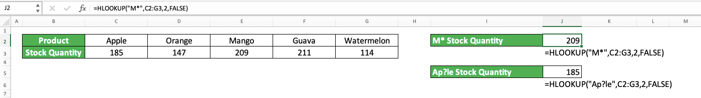
In the example, we use * and ? in the lookup reference value inputs of our HLOOKUPs. As you can see, they can help us to find the data we want through their capability to represent any character.
When we utilize them in the right way, they can surely become handy to help write the perfect HLOOKUP for us.
A Better Alternative to HLOOKUP? HLOOKUP vs INDEX MATCH
If you often use HLOOKUP to find data in excel, then you might want to consider an alternative method. The method uses the INDEX MATCH formulas combination and it is more flexible in terms of its data lookup process.INDEX can help us to get data by inputting the data row and column positions in a cell range. Meanwhile, MATCH can help us to get the row or column position of data in a cell range. When we combine them, we can get a powerful lookup formula that can find data horizontally or vertically.
The combination can certainly replace the use of HLOOKUP and VLOOKUP too. You don’t need to switch between formulas depending on your reference table form if you use INDEX MATCH.
The general writing form of INDEX MATCH in excel as an HLOOKUP alternative is as follows.
= INDEX ( reference_cell_range , row_position , MATCH ( lookup_reference , lookup_reference_range , lookup_mode ) )
MATCH helps us to find the column position we need for our INDEX. It will work just like HLOOKUP. You can use MATCH to find the row position too if you need it.
To compare between HLOOKUP and INDEX MATCH, here is a table that has some of the comparison points.
| HLOOKUP | INDEX MATCH |
|---|---|
| Find data horizontally (by rows) | Find data vertically and/or horizontally (by columns and/or rows) |
| The lookup reference value needs to be in the first row of the reference table | The lookup reference value can be in any row of the reference table |
| Lookup mode options are an approximate match (smaller nearest) and exact match | Lookup mode options are an approximate match (smaller nearest and larger nearest) and exact match |
| You only need to master one formula (if you don’t need to use VLOOKUP) | You need to master two formulas to use INDEX MATCH as it consists of INDEX and MATCH |
Here is the implementation of INDEX MATCH in excel which mirrors HLOOKUP.
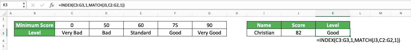
Here, we use the same data set as the one we use for the HLOOKUP implementation example early in this tutorial. As we use the INDEX MATCH like an HLOOKUP, we put our MATCH in the INDEX column position input part.
We input the row cell range where we want to get our result to the INDEX’s cell range input part. As it has only one row, we give 1 to the INDEX row position input part.
In MATCH, we input our lookup reference value and the row cell range where we should find it. As we want the smaller nearest approximate match here (mirrors the TRUE lookup mode of HLOOKUP), we give 1 as the lookup mode input of our MATCH.
By writing it correctly, INDEX MATCH can have a similar capability to HLOOKUP! If you have time, then you should learn how to master INDEX MATCH. Doing so should give you a strong HLOOKUP alternative to use in your excel work!
Exercise
After learning how to use the HLOOKUP excel formula completely, now is the time to do an exercise. You should do it so you can deepen your understanding of the HLOOKUP implementation in excel.Download the exercise file below and answer all the questions. Download the answer key file if you have done the exercise and want to check your answers. Or probably when you are confused about how to answer all the questions.
Link to the exercise file:
Download here
Questions
Answer each question with HLOOKUP in the appropriate gray-colored cells!- What is the number in column E on the row marked with 6?
- What is the number in column C on the row marked with 1?
- What is the number in the column with a number close to 60000 on the row marked with 5? Find the number in the row marked with 10
Link to the answer key file:
Download here
Additional Note
To add a literal * or ? in your HLOOKUP lookup reference value, you need to write a tilde symbol ( ~ ) just before it. Not writing a tilde symbol will cause HLOOKUP to recognize your * or ? as wildcard characters.Related tutorials you should learn: