How to Find Duplicates in Excel
Home >> Excel Tutorials from Compute Expert >> Excel Tips and Trick >> How to Find Duplicates in Excel
In this tutorial, you will learn how to find duplicates in excel using various methods.
When processing data in excel, we sometimes need to find duplicates to mark, revise, or delete. This is so they don’t affect negatively the further work that we do in excel.
We can find those duplicates using the conditional formatting feature or by utilizing the formulas in excel. After learning from this tutorial, you should be able to practice those methods smoothly yourself.
Disclaimer: This post may contain affiliate links from which we earn commission from qualifying purchases/actions at no additional cost for you. Learn more
Want to work faster and easier in Excel? Install and use Excel add-ins! Read this article to know the best Excel add-ins to use according to us!
Table of Contents:
How to Find Duplicates in Excel Using Conditional Formatting
The first method to find duplicates in excel is by using the conditional formatting feature.Conditional formatting has a special menu to identify the duplicates we have in an excel cell range. That makes it easier for us to find duplicates using this feature.
The steps to utilize this method are pretty simple too and you should be able to master it fast. We will explain the steps below with an example to help you understand them better.
For the example itself, let’s say we have a data table like this in our excel file.
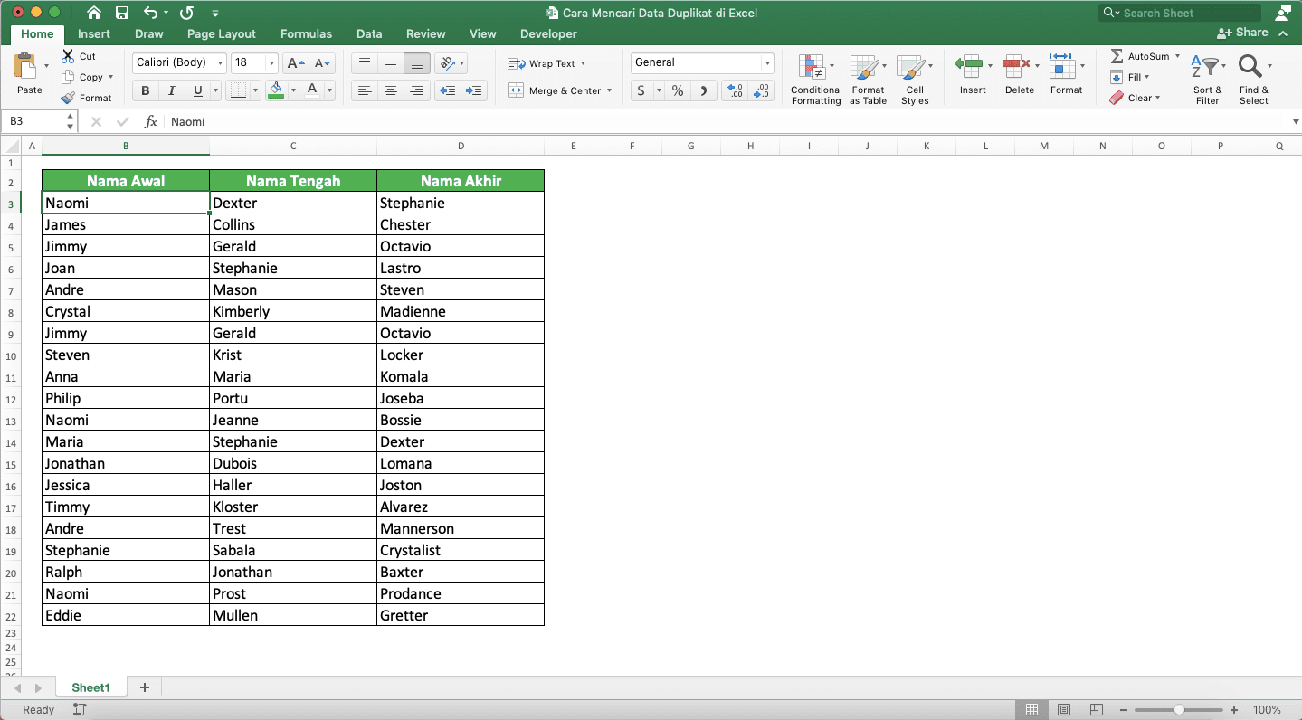
Say we want to identify the duplicates in the “First Name” column there. How do we do it using conditional formatting?
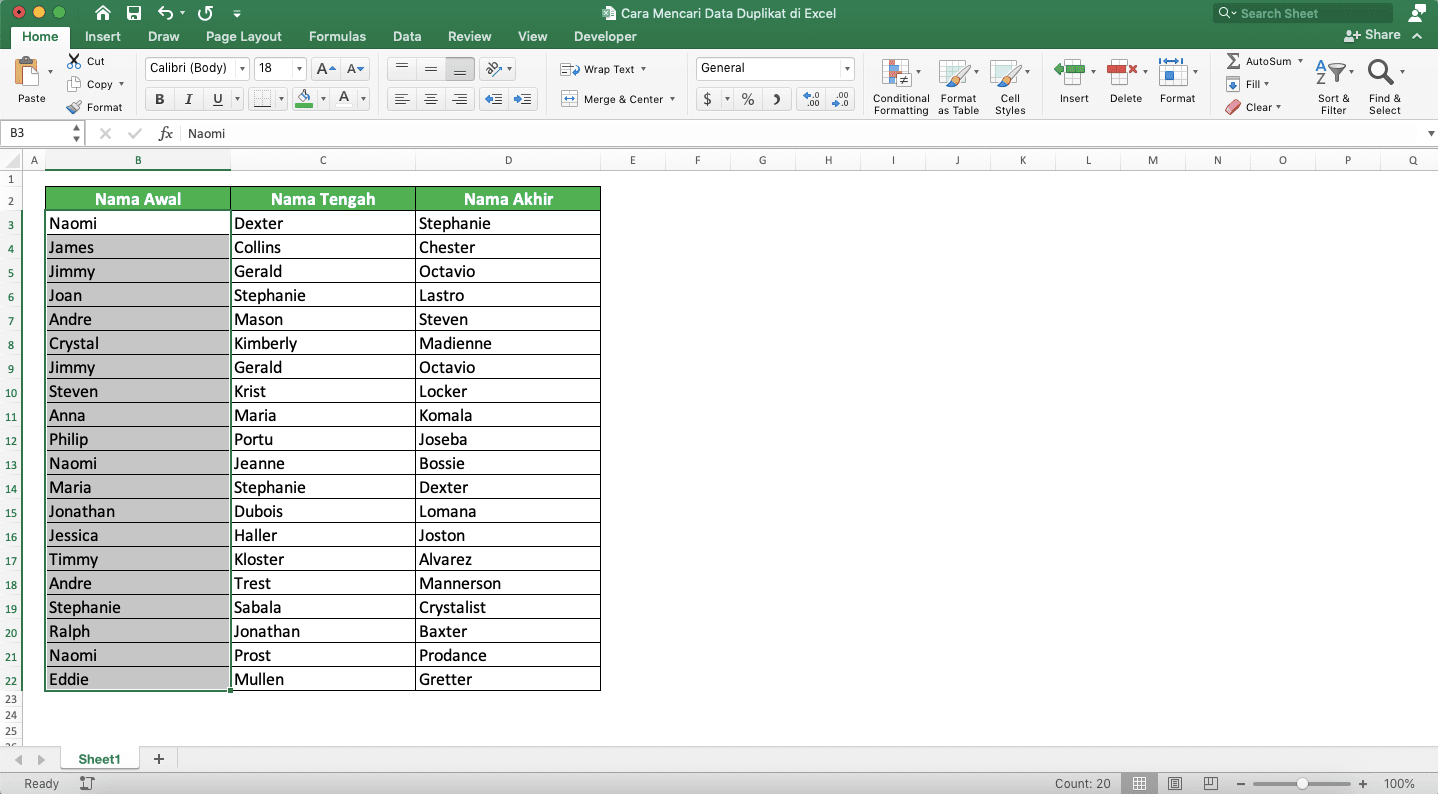
First, you need to highlight the cell range where you want to check the duplicates on. In the example, that means we highlight the data in the first name column in our data table.
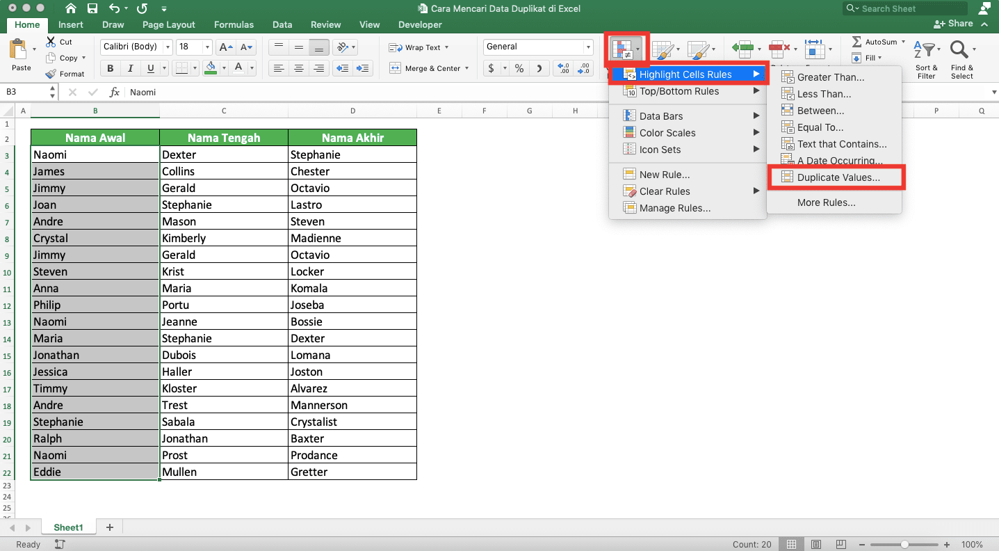
Then, click on the Conditional Formatting button in the Home tab. Put your pointer on the Highlight Cell Rules choice in the list shown.
This will show other choices inside the Highlight Cell Rules choice. Click the one with the Duplicate Values… label on it.
Excel will show you the New Formatting Rule dialog box. Make sure the dropdown there indicates that you want to mark the duplicates in your cell range.
You can also modify the marking style on your duplicates by choosing it from the Format with… dropdown.

After you have chosen, click OK. The duplicates on your cell range will have been highlighted using the style you choose!
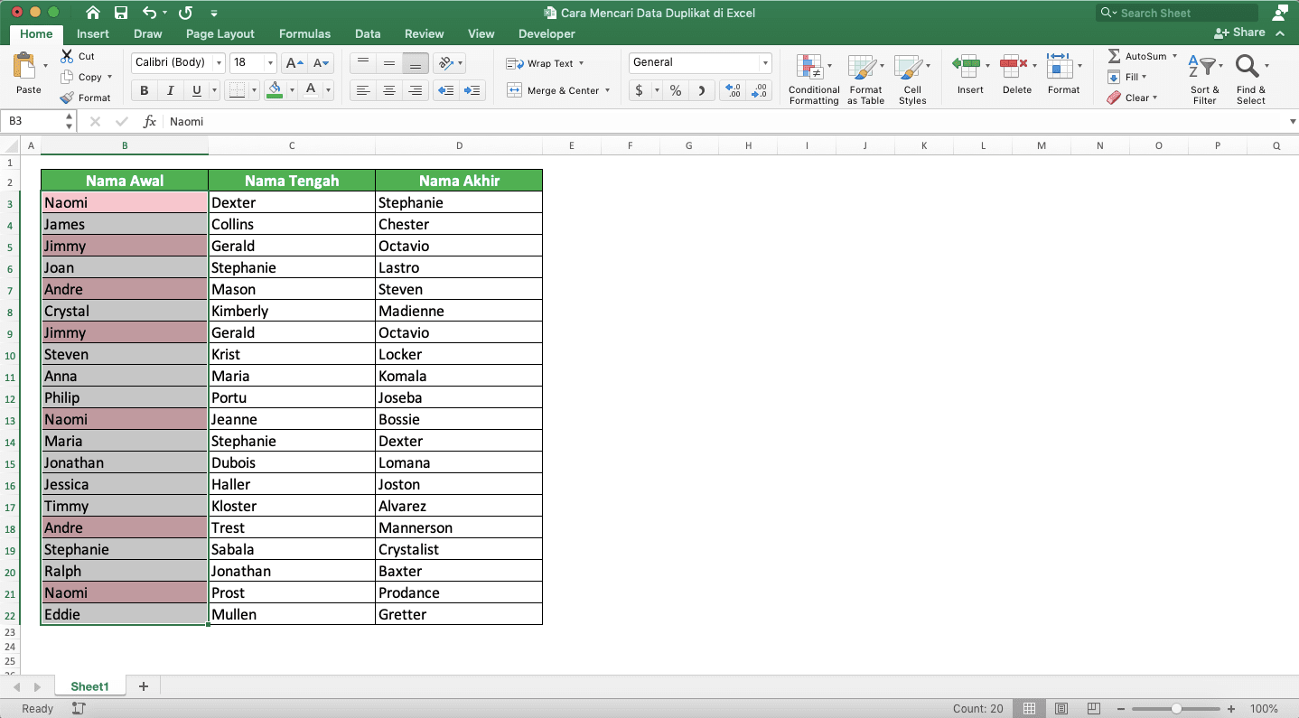
It is pretty easy to use the conditional formatting to identify those duplicates, right? Use conditional formatting if you prefer it compared to the other methods given in this tutorial!
How to Find Duplicates in Excel Using COUNTIF
Besides conditional formatting, you can also use excel formulas to help you find duplicates in your data. One of the formulas you can use for that is COUNTIF.To use COUNTIF, you need to set a helper column that will serve as the marks of your duplicates. Make that helper column in parallel and the same size as your data cell range. You will write some COUNTIFs in that helper column which will help identify the duplicates in your cell range.
In general, the COUNTIF you write for that will be as follows.
=COUNTIF(data_cell_range, data_to_check_for_duplicates) > 1
Input the cell range which contains all the data where you want to identify the duplicates of to your COUNTIF. Then, input the cell which is in parallel with the cell in the helper column where you currently type your COUNTIF. Write this COUNTIF in the first cell of your helper column.
Don’t forget to add dollar symbols in front of your row and column coordinates in your COUNTIF cell range input. This is so you can easily copy your COUNTIF later to other cells in your helper column after you write one.
After that, don’t forget to write the “>1” condition after you write your COUNTIF. This is to check whether there is a duplicate for the data that becomes your COUNTIF input.
If the COUNTIF result is more than one, then your formula result becomes TRUE, meaning there is at least one duplicate. If FALSE, then there is no duplicate for the data.
Get the TRUE and FALSE from all the data in your cell range using this formula. You will identify the duplicates in your cell range in no time!
If you want, then you can also label your duplicates with your own text (not TRUE/FALSE) by combining COUNTIF with IF. We can write the COUNTIF and IF combination as follows.
=IF(COUNTIF(data_cell_range, data_to_check_for_duplicates)>1, “Duplicates”, “Not Duplicates”)
You can change the “Duplicates” and “Not Duplicates” there with the labels you prefer.
To understand easier about the COUNTIF use to find duplicates in excel, look at the screenshots below.
COUNTIF:

IF COUNTIF:

You can check the formula writing for each screenshot in the formula bar. As you can see, we set up a helper column to be the place where we write our COUNTIF.
In these screenshots, we try to identify the duplicates in the “First Name” column. For that, we write a COUNTIF in the first row of the helper column. The COUNTIF inputs are the cell range of the “First Name” column and the first row’s first name.
We also write the condition “>1” after the COUNTIF to get the duplicate result from our formula.
The screenshots also show the difference of using only COUNTIF and using COUNTIF with IF. If we only use COUNTIF, then the duplicates will be marked with TRUE logic values. If we use COUNTIF with IF, then we can label them the way that we want.
After we write COUNTIF in the first row, just copy the formula down until it can check all of our data. We will then get the duplicate marks for those data immediately!
How to Find Duplicates in Two Columns in Excel Using VLOOKUP
What if we want to check the duplicates of one column data in another column? What method can we use to do that kind of checking process?Well, we can use the VLOOKUP formula for that. It will check whether there is the data of one column in another column and will return the result to you.
The general writing of VLOOKUP to do that for us is as follows.
=VLOOKUP(data_from_column_1, column_2_cell_range, 1, FALSE)
In the VLOOKUP, we input the data that we want to check the duplicates of as the lookup value. The column where we want to check the duplicates will become the cell range input.
We input 1 as the result column index because we only have one column in our VLOOKUP cell range input. Moreover, we input FALSE as the lookup mode because we want an exact match to make sure there is a duplicate.
The result of that VLOOKUP writing will be the data or an error if the duplicate isn’t found. To make the result better, we can use IF and ISERROR to give the labels that we want.
Generally, we can write a combination of those three formulas like this.
=IF(ISERROR(VLOOKUP(data_from_column_1, column_2_cell_range, 1, FALSE)), “Not Duplicates”, “Duplicates”)
If the VLOOKUP doesn’t produce an error, then that means there is a duplicate in that other column. The ISERROR result will become FALSE. If there isn’t a duplicate, then the result will become TRUE.
We can give the not duplicate/duplicate labels as we prefer in the IF. You can change the “Not Duplicates” and “Duplicates” in the writing there to do it.
The example of the VLOOKUP implementation to find duplicates in excel is as follows.

You can see the formula writing in the screenshot’s formula bar. We write the IF ISERROR VLOOKUP combination in one column to check the first name duplicates in the middle name column.
We input the first name data and the middle name column in the VLOOKUP there. We check the VLOOKUP result using ISERROR and label the duplicate checking result using IF.
Don’t forget to add dollar symbols in the VLOOKUP’s cell range input. This is to make it much easier to get the formula we write to other cells that need it.
Write the formula combination correctly and you will get the results you want (as you can see in the screenshot)!
How to Find Duplicates in Two Columns per Row
We probably want to check the duplicates in two columns but the duplicates must be in the same row. If we have that kind of condition, then we can utilize the equal symbol on our keyboard to check it.We write the formula with the help of an equal symbol like this.
=column_1_data = column_2_data
Both columns’ data should be parallel to make it easier for us when looking at the results.
The formula writing will produce TRUE if they are duplicates and FALSE if they aren’t duplicates. If you want to label the duplicates/non-duplicates, then you can add IF in your writing.
=IF(column_1_data = column_2_data, “Duplicates”, “Not Duplicates”)
As always, you can change the “Duplicates” and “Not Duplicates” there into the labels you prefer.
The example of the writing in action is as follows.
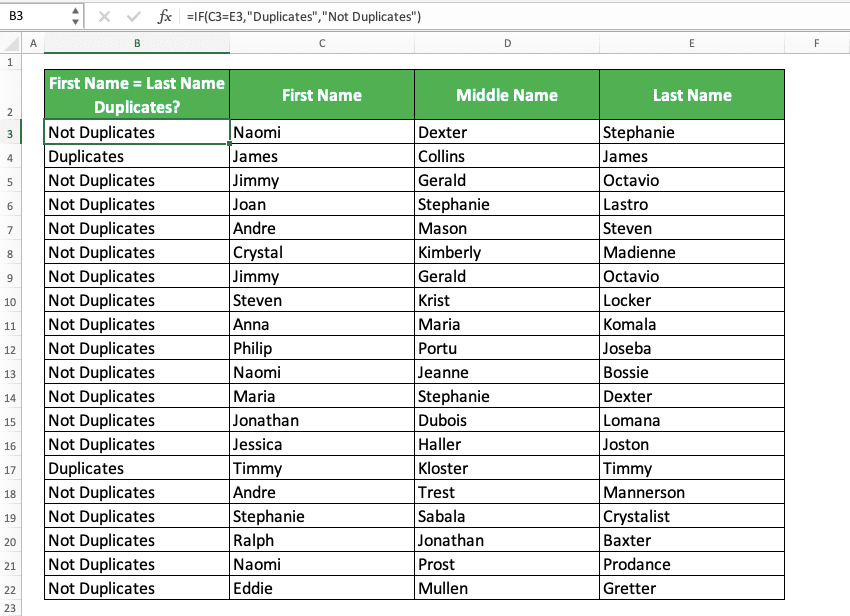
As you can see, we check the duplicates in each row of the first name and last name in the example. For that, we input the first name, equal symbol, and last name in the first input of IF. The inputs of the first name and last name are parallel with each other.
Next, we input the label we want for the duplicates/non-duplicates. Enter and we will get the duplicate checking result from our formula!
For the other rows in the columns, just copy the formula we have written for the first pair of data. If the columns are in the same size and parallel with each other (as normally they are), then that should be enough.
How to Find Row Duplicates in Excel
What if we want to check the duplicates of one row of data in its entirety? Meaning that if one column in the row isn’t the same as another row, then it won’t count as a duplicate.We can do the duplicates checking for that by concatenating all the column data for each row first. After that, we can check the duplicates by using conditional formatting or COUNTIF method.
This will be easier to explain with an example. For that, let’s have the name data table again that we have used few times previously.
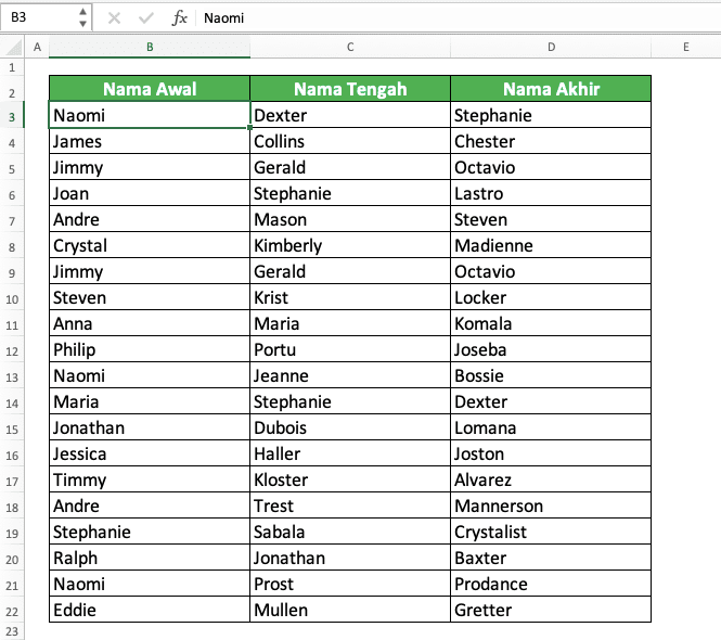
We want to count the duplicates of the full names there. How can we do that?
We first set up a helper column that is in line with the other columns that contain our data.

Then, we concatenate all the data we want as part of the rows we need to check the duplicates from. We can concatenate them using the CONCATENATE/CONCAT formula or the ampersand symbol (&).
In this example, we use the ampersand symbol to help us. To use it, put all the data we want to concatenate with the ampersand symbol in between each of them.
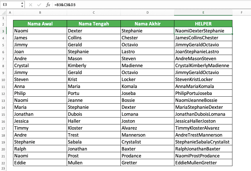
You can see how we concatenate the data in the formula bar.
Next, we can check the rows which have duplicates from the helper column. You can use the conditional formatting or COUNTIF method for that.
These are the results for both methods if we use them in our example.
Conditional Formatting:
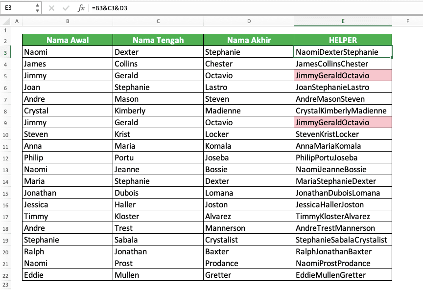
COUNTIF:

Both methods will mark the duplicates in our rows. Thus, we can find them as we need them to be!
Exercise
After you have learned how to find duplicates in excel using various methods, let’s do an exercise! This is so you can understand your learnings more practically.Download the exercise file and do the instructions below. Download the answer key file too if you have done the exercise and want to check your answers. Or probably when you are confused about how to do the instructions!
Link to the exercise file:
Download here
Instructions
Answer these questions on their appropriate sheets according to their numbers! (1 = Sheet1, 2 = Sheet2, 3 = Sheet3)- Find the duplicates in the name column using conditional formatting! Mark the duplicates with yellow cell color and red font color!
- Find the duplicates in the age column using COUNTIF! Mark the duplicates with TRUE and the non-duplicates with FALSE!
- Find the row duplicates in the table data (using conditional formatting or COUNTIF)!
Link to the answer key file:
Download here
Additional Note
Conditional formatting, COUNTIF, and VLOOKUP aren’t case-sensitive when they check for duplicates in your cell range.Other tutorials you should learn:


